By Xinyong
EMR Jindo is a cloud-native engine for online analytical processing (OLAP) launched by Alibaba Cloud E-MapReduce (EMR). With this engine, EMR was the first cloud-based TPC-DS contestant to submit its results. After continuous kernel optimization, EMR significantly improved its TPC-DS performance to 3615071 by using the latest EMR Jindo engine, while reducing the cost to RMB 0.76.
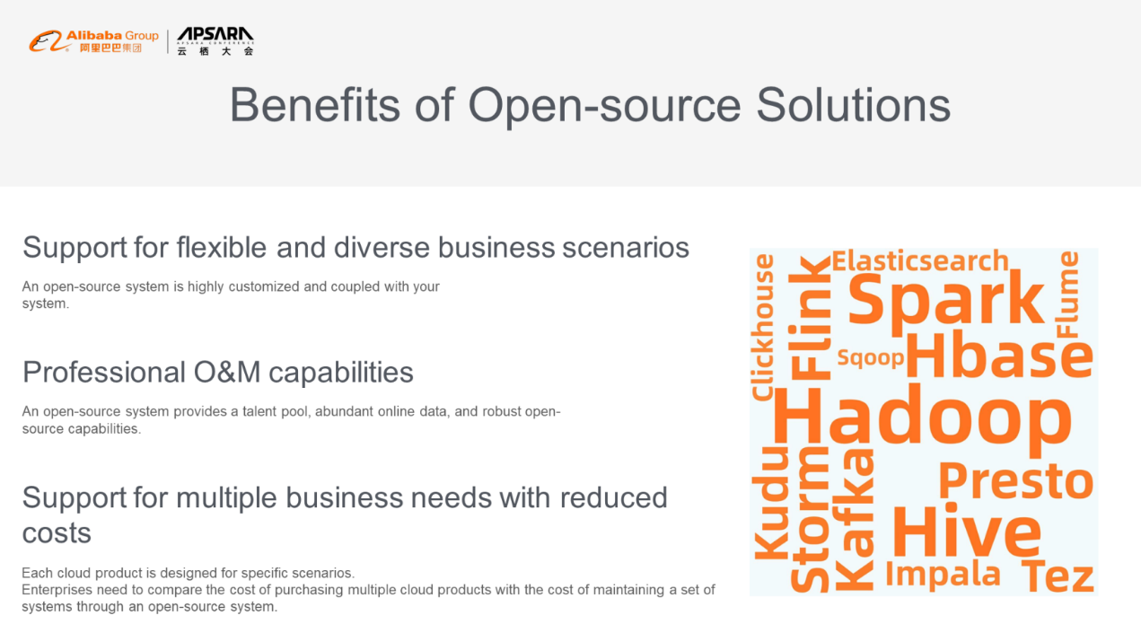
At the big data technology session of the 2019 Apsara Conference held in Hangzhou, Xinyong, an EMR technology expert from the Alibaba Computing Platform Division of Alibaba Cloud, shared his knowledge about how to build a cloud-based EMR platform for data analytics by using an open-source system. He also discussed the technologies used to develop the EMR Jindo engine and the cloud-based big data architecture solution based on EMR Jindo.
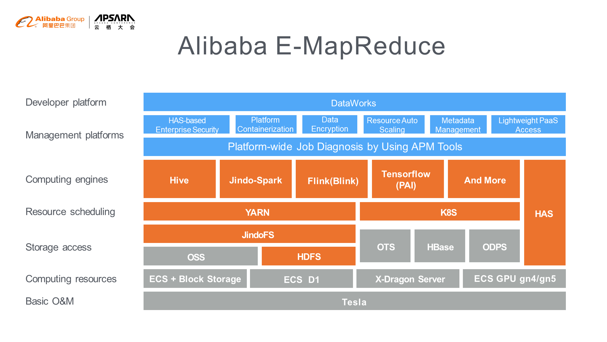
The following figure shows the architecture of EMR.
You can migrate your data to the cloud through one of two methods:
(1) Purchase Elastic Compute Service (ECS) resources to build an open-source system
(2) Use EMR. It is complicated to build an open-source big data system from scratch because this system involves many components, such as Spark, Hive, Flink, and TensorFlow. In addition, this system may consist of hundreds of clusters, which poses great challenges to O&M.
EMR provides the following advantages:
(1) EMR is an out-of-the-box service that supports convenient automatic deployment and component configuration. It automatically recommends and tunes parameter settings based on your server type.
(2) EMR is integrated with other Alibaba Cloud services. For example, after you store data in Object Storage Service (OSS), EMR can directly read the data from OSS without needing to configure authentication.
(3) EMR integrates many proprietary plug-ins, which are unavailable in other Alibaba Cloud services.
(4) EMR provides components that are both compatible with and superior to open-source components. For example, the Flink component integrates Blink and TensorFlow (also available in Machine Learning Platform for AI) independently developed by Alibaba Cloud. This is one of the contributions that Alibaba Cloud has made to the open-source community in order to provide its technologies to external users.
(5) EMR provides an application performance management (APM) component used for platform-wide job diagnosis and alerts. This component implements automatic O&M, allowing you to more conveniently operate your clusters.
(6) EMR is integrated with DataWorks. You can use some simple features of EMR through DataWorks.
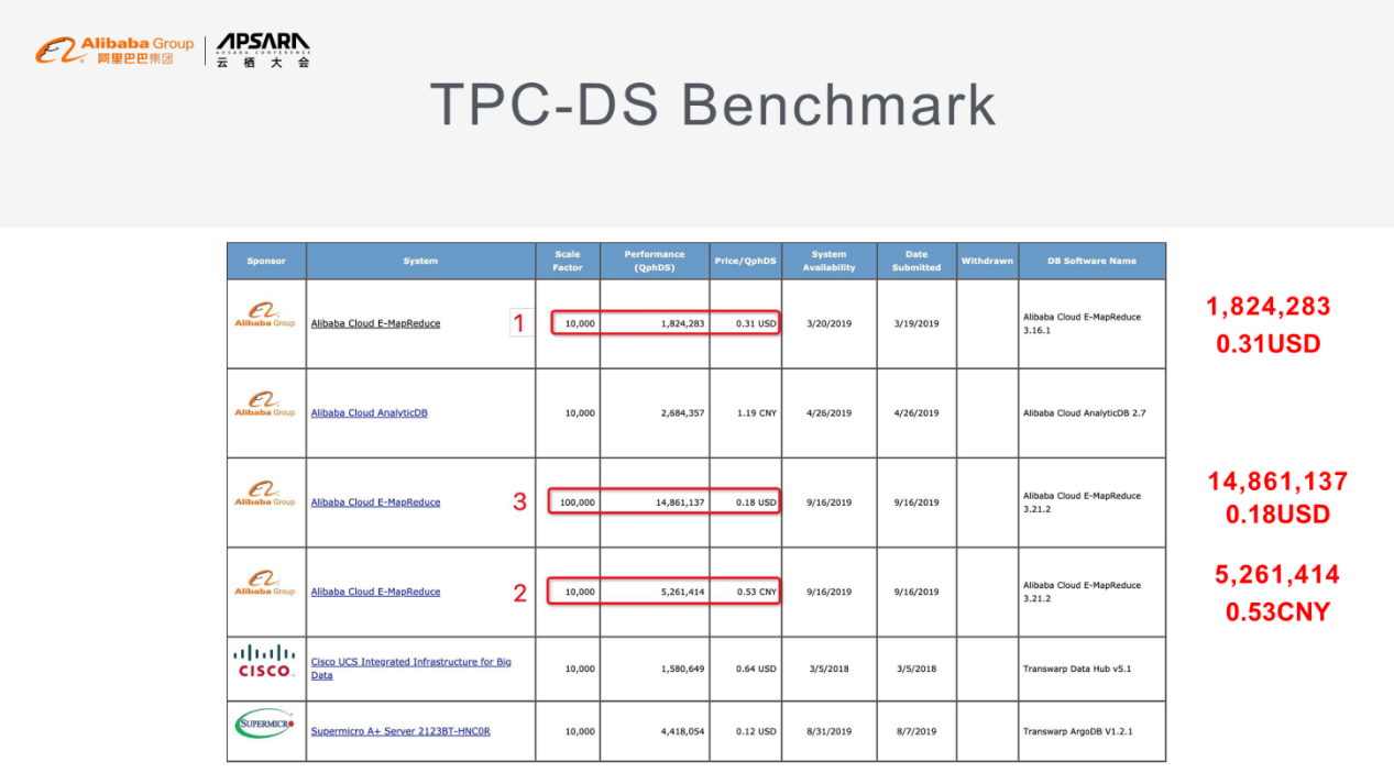
The following figure shows a TPC-DS benchmark test report. In the 10 TB testing conducted in March 2019, EMR achieved a performance score of about 1,820,000 at a cost of USD 0.31. In another 10 TB testing conducted in October 2019, EMR achieved a performance score of 5,260,000 at a cost of RMB 0.53. This means the EMR performance was improved by a factor of 2.9 over a period of half a year and the cost was reduced by 1/4. Alibaba was the first vendor to submit a 100 TB test report to TPC-DS. These achievements would not have been possible without the support of the EMR Jindo engine.
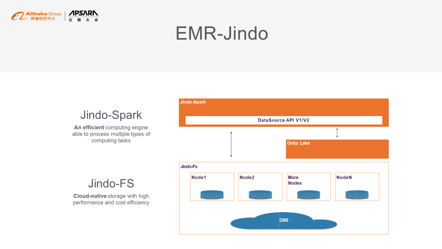
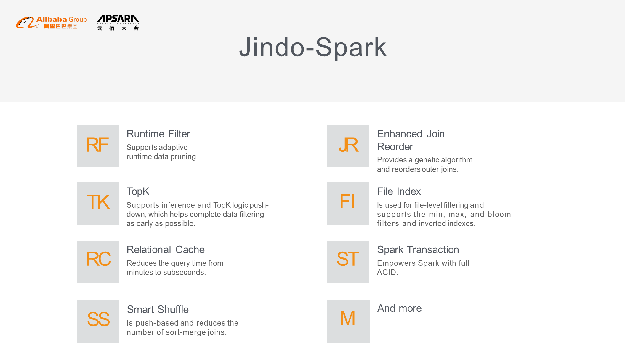
The Jindo Spark computing engine provides a range of Spark optimizations. For example, runtime filters support adaptive runtime data pruning. The enhanced join reorder feature is designed to solve the problem of outer join reordering. TopK supports inference and TopK logic push-down, which helps perform data filtering earlier. File indexes can be used for file-level filtering and support the min, max, and bloom filters and inverted indexes. The proprietary relational cache uses a single engine to reduce the query time from minutes to less than a second. The scenario-based Spark transaction feature was introduced to empower Spark with full atomicity, consistency, isolation, and durability (ACID). Finally, the smart shuffle feature can reduce the number of underlying sort-merge joins, which improves the shuffle efficiency.
Runtime filters work in a similar way to the dynamic partition pruning (DPP) feature of Spark but provide more powerful functions. DPP can process analytical tables, whereas runtime filters can process both analytical and non-analytical tables. Runtime filters are used to dynamically prune runtime data to avoid unnecessary computing. For example, in a join query, data cannot be filtered by means of pushing values down to the storage layer. The final data magnitude cannot be predicted during logical estimation. If the join query involves analytical tables, the runtime filter first estimates the volume of data to be joined in one of the tables. If the data volume is small, the runtime filter screens the data and pushes the data to the other table for filtering. If the join query involves non-analytical tables, another type of filter, such as the bloom filter, is introduced to collect min or max statistics.
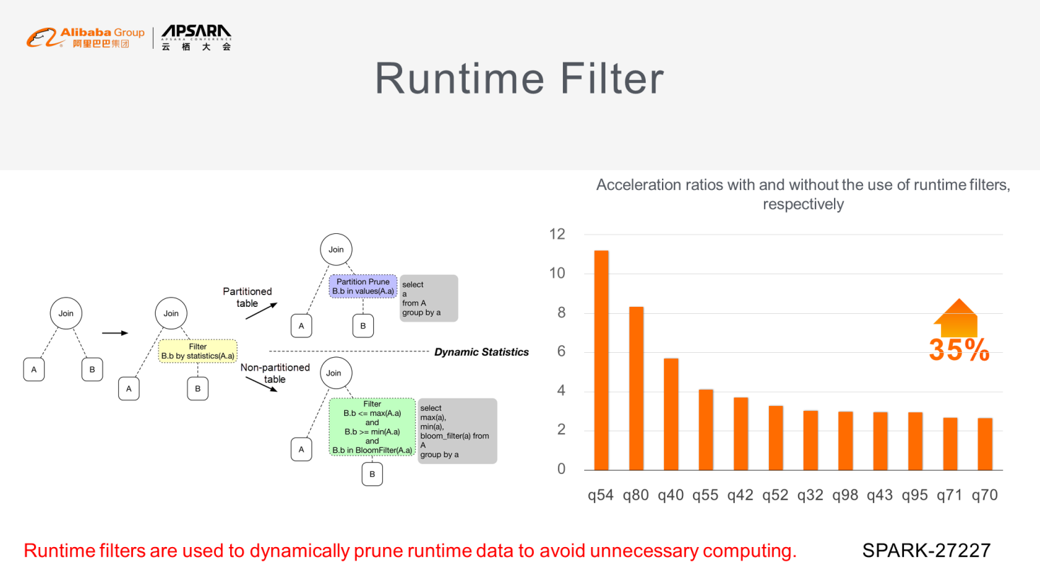
Based on these statistics, the system extracts data from the table with less candidate data and pushes the data to the other table for filtering. Runtime filters are highly cost-efficient. They can significantly improve performance through simple evaluation in an optimizer. As shown in the following figure, runtime filters improve performance by about 35%. The runtime filter feature has been submitted to Spark PR (Spark-27227).
The execution order of operators can significantly affect the execution efficiency of SQL queries. To minimize this impact, we can execute operators in a different order to complete data filtering as early as possible.
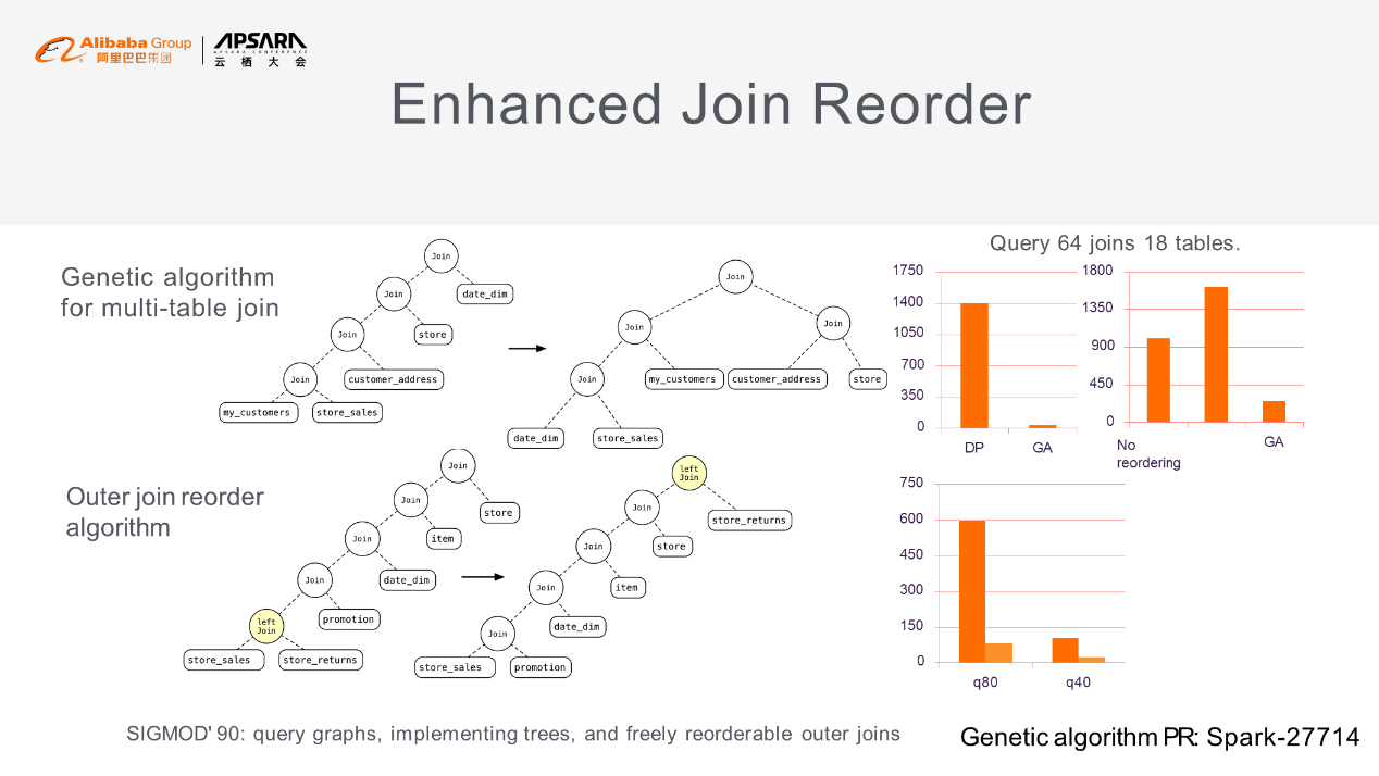
Let's look at the example shown in the upper-left corner of the following figure. If the two underlying tables are very big, joining the two tables results in high overhead. If we continue to join the resulting big data with small tables, the big data is passed on layer by layer. This affects the join efficiency. One solution is to filter out irrelevant data in the big tables to reduce the volume of data that is passed downstream. To implement this solution, Spark provides a dynamic planning algorithm. However, this algorithm is only applicable to joins of no more than 12 tables. To join more tables and even hundreds of tables, EMR provides a genetic algorithm, which linearly reduces the 2n complexity of the dynamic planning algorithm.
Let's look at the example shown in the upper-right corner of the following figure. Query 64 involves an operation that joins 18 tables. The join takes 1,400 seconds when using the dynamic planning algorithm, but takes only about 20 seconds when using the genetic algorithm. The join reorder feature provides the outer join reorder algorithm. SQL does not support random reordering of outer joins, but this does not mean outer joins cannot be reordered. For example, the predefined order "A left join B -> Left join C" can be changed under certain conditions. Spark does not consider outer join optimization, whereas EMR determines the necessary and sufficient conditions for outer join reordering based on existing studies. The example shown in the lower-left corner of the following figure uses the outer join reorder algorithm. The chart in the lower-right corner of the figure shows the improvement of outer join efficiency when using this algorithm.
The native cache of Spark has several limitations. One limitation is that this cache is applicable at the session level. If a query fragment is frequently used, a cache is created for the related session. When the session ends, the cache disappears. Another limitation is that the Spark cache cannot be used across different devices because it stores data on the local device rather than in distributed mode. Based on the Spark cache, EMR provides the relational cache feature. It creates a cache for any data entity abstracted from relational data, such as Spark tables, views, and datasets. The created cache is similar to a materialized view but provides more advantages. These advantages include response to a multidimensional online analytical processing (MOLAP) engine in subseconds, interactive business intelligence (BI) and dashboards, data synchronization, and data pre-organization.
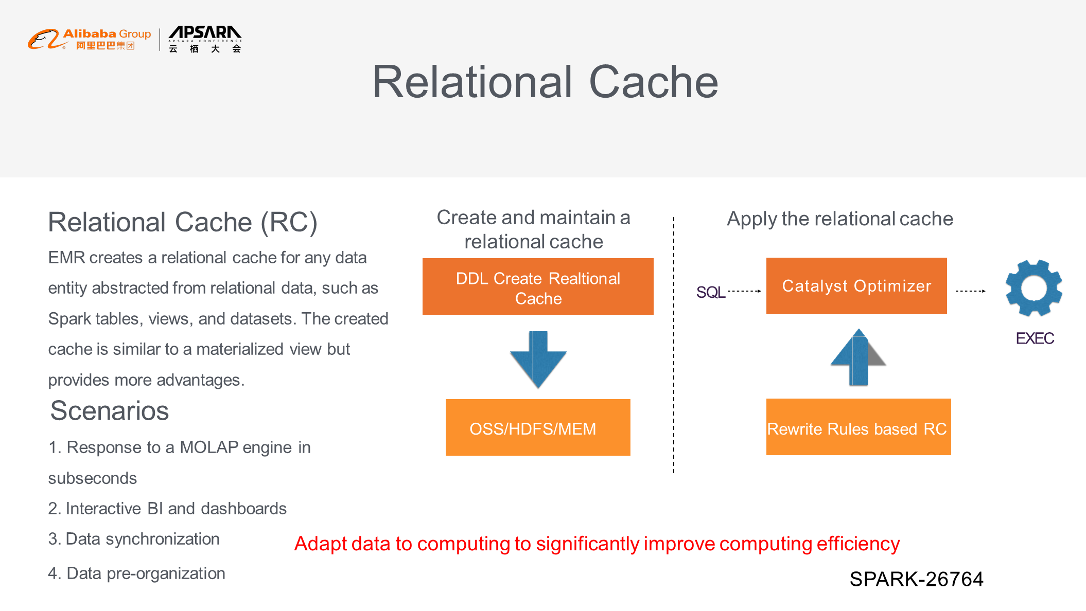
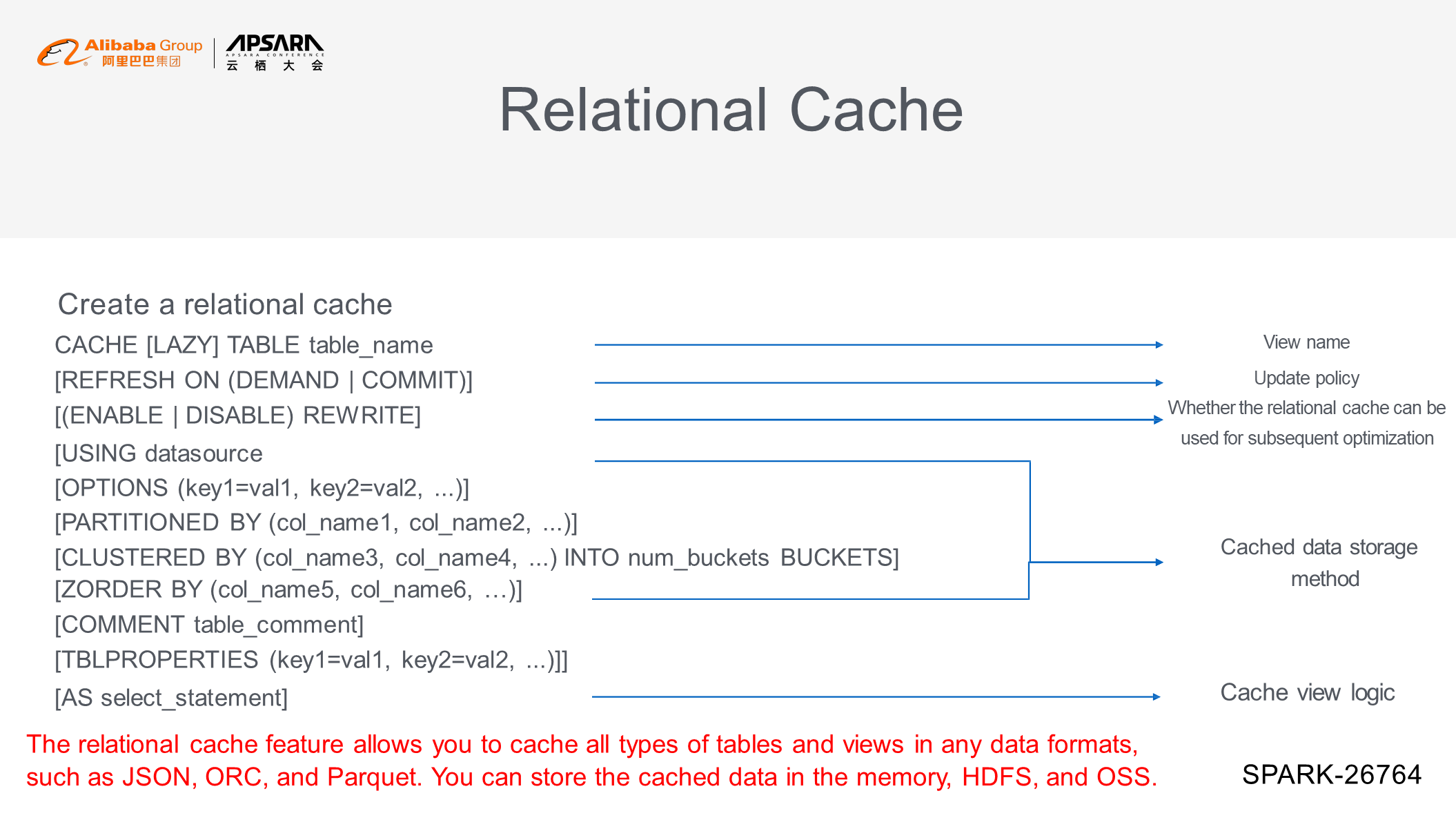
The following figure shows the process of creating a relational cache. Its syntax is similar to the data definition language (DDL) of Spark SQL. After you cache a table or a view, you can specify the following settings: an update policy (options: DEMAND and COMMIT) for the relational cache, whether the relational cache can be used for subsequent optimization, cached data storage method, and cache view logic. The relational cache feature allows you to cache all types of tables and views in any data format, such as JSON, ORC, and Parquet. You can store the cached data in the memory, HDFS, and OSS.
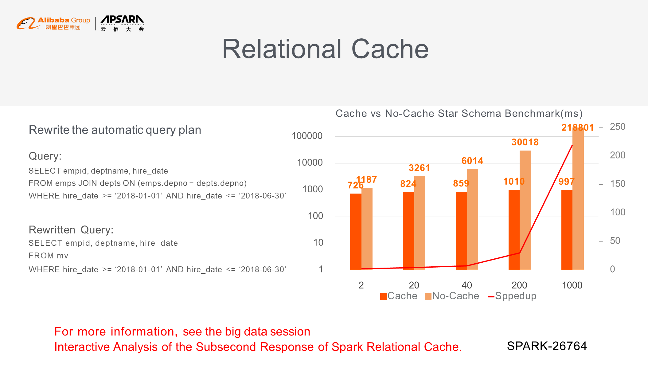
The relational cache can optimize the SQL queries that you enter. The native SQL cache of Spark is only applicable to manually entered SQL queries that exactly match the cache. The relational cache works in a different way. For example, a cache is created when the four tables a, b, c, and d are joined. Then, when the three tables a, b, and e are joined, the results of joining tables a and b can be read from the four-table join cache. The chart in the right part of the following figure compares the results of a benchmark test that uses the relational cache with the non-cache test results. The relational cache keeps the response time under a second.
For more information, see Interactive Analysis of Subsecond Response of Spark Relational Cache.
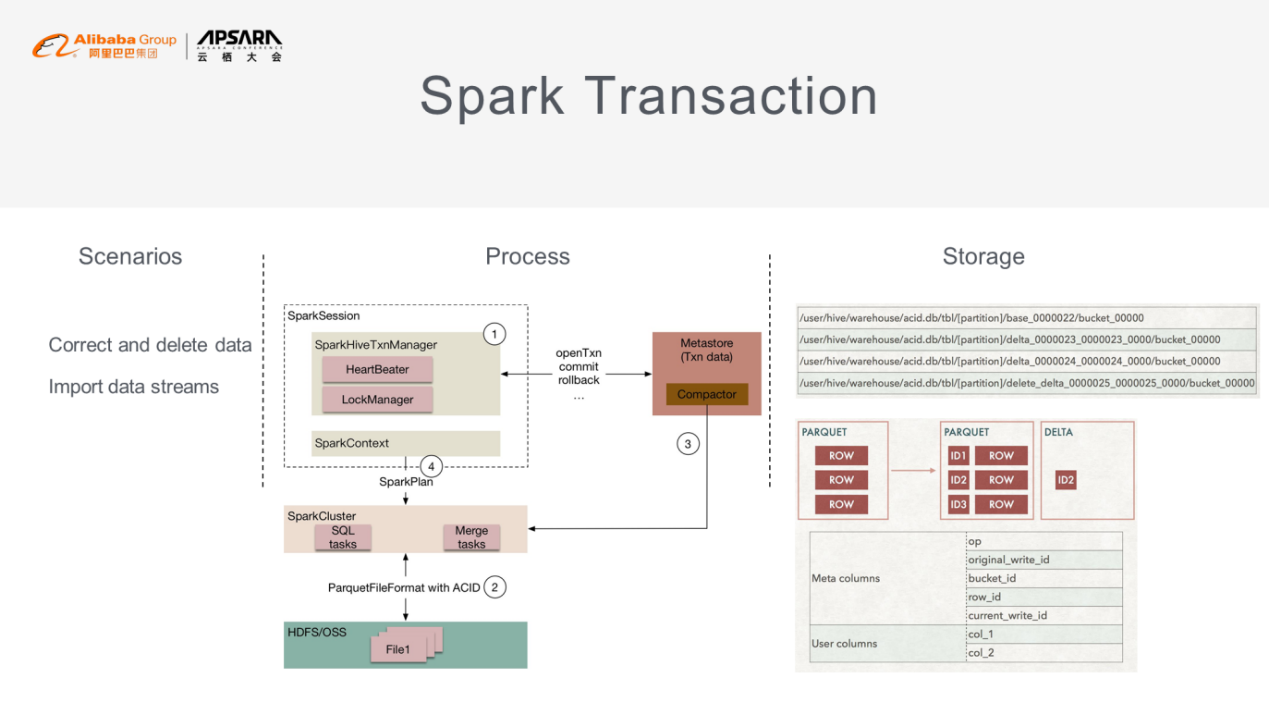
Data is typically imported in batches. For example, data is imported once every day. However, when you import streaming data, raw data is written in real time without processing. If you want to delete or update the imported data, you can use the Spark transaction feature. This feature is generally a lock-based implementation of Multi-Version Concurrency Control (MVCC), which depends on the underlying storage.
Given Hive-Spark compatibility, big data is stored as files in directories, and file versions are controlled based on rows. Once data is written to a row, this row is assigned a unique meta column for identification, such as OP, original_write ID, bucket ID, and row ID. When you update a row, this row is not updated in situ but is taken out for writing new data. Then, a new version of this row is generated and stored. When you read data from a row, the data from multiple versions of this row is merged before it is returned to you.
EMR introduced the local disk model early on. This model was used to deploy clusters in a way similar to the deployment of big data releases in an on-premises cluster. This deployment method was costly. In addition, it was difficult to dynamically scale local storage in and out due to the metadata bottleneck of HDFS at that time. One solution is to separate computing and storage, with data stored in OSS. However, this solution causes performance degradation for two reasons. One reason is that it is time-consuming to operate metadata in OSS. The other reason is that performance is seriously affected by the transmission bandwidth used to read data across networks.
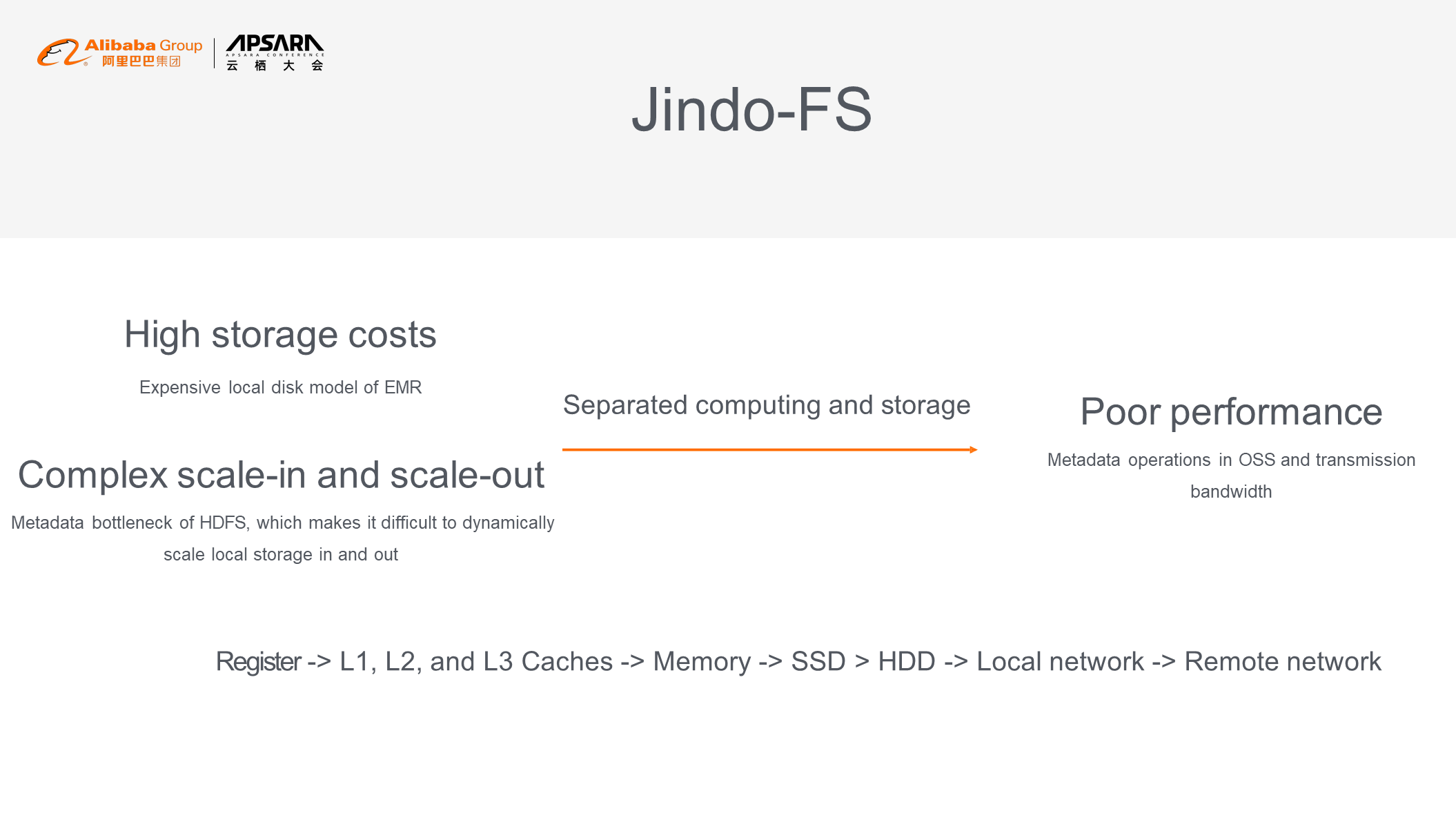
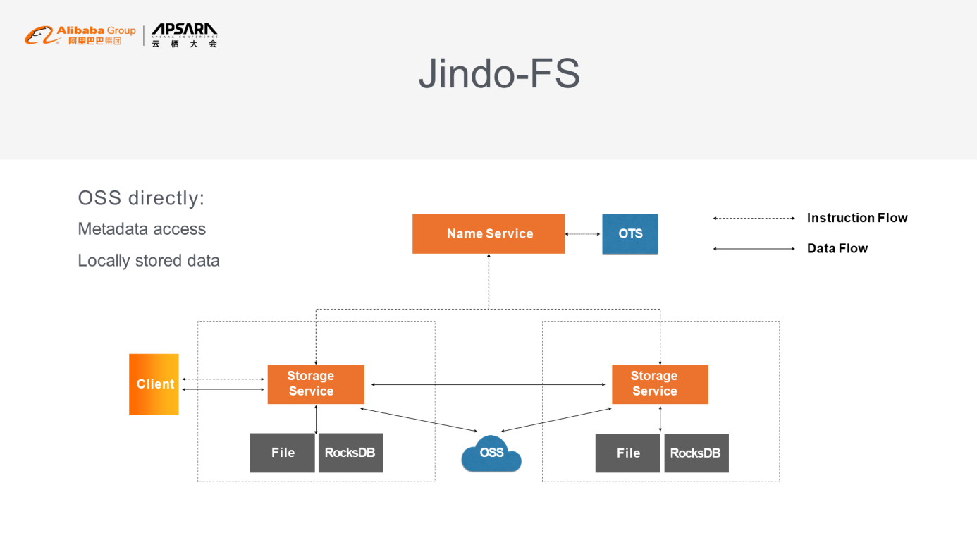
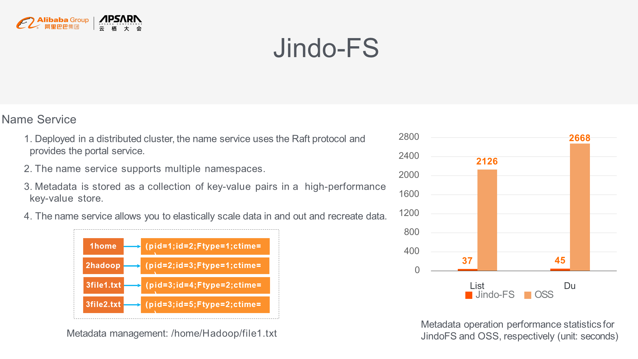
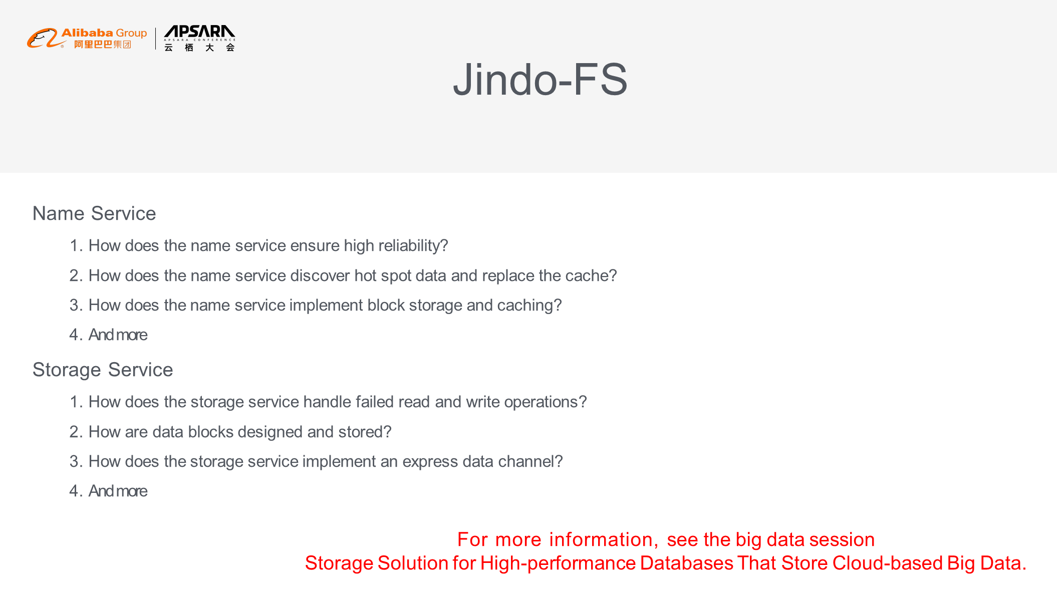
To avoid performance degradation, JindoFS pulls data from the remote end to the computing side for caching. JindoFS is similar to HDFS, and its architecture is similar to the primary-secondary architecture. JindoFS consists of the name service and storage service. JindoFS can cache frequently accessed tables in RocksDB at multiple layers. The name service can be viewed as a primary node of JindoFS, but it is different from a primary node of HDFS. Deployed in a distributed cluster, the name service uses the Raft protocol and provides the portal service and multi-namespace support. Metadata is stored as a collection of key-value pairs in a high-performance key-value store. In reality, data is stored in OSS and Tablestore rather than in the name service. Therefore, the name service allows you to elastically scale data in and out, release data, and recreate data.
JindoFS provides the underlying metadata management feature. It splits data into a collection of key-value pairs, which are assigned incremental IDs and queried layer by layer. For example, when you read the data in /home/Hadoop/file1.txt, the system reads data from Tablestore only three times. The chart in the right part of the following figure shows the test results, indicating JindoFS performs better than OSS in terms of metadata operations.
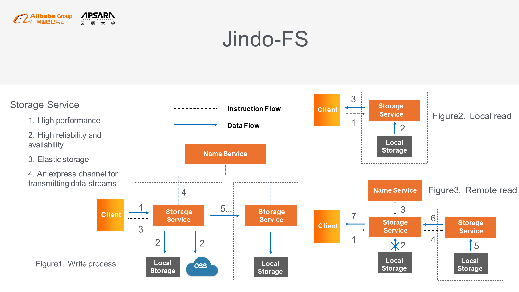
JindoFS uses the storage service for underlying storage. When you write data, the storage service stores the file to be written in both local storage and OSS, and then returns the writing results to you. At the same time, the storage service transmits data replicas between cluster nodes. The read process is similar to that in HDFS. If the data to be read matches locally stored data, the data is read from local storage. Otherwise, the data is read from the remote end. The storage service features high performance, reliability, availability, and elasticity. To support high performance, JindoFS creates an express channel for transmitting data streams and provides a range of policies, such as the policy used to reduce the number of times data is copied in the memory.
For more information, see the article Introducing JindoFS: A High-performance Data Lake Storage Solution. This article provides more information about the name service and storage service of JindoFS, such as (1) how the namespace service ensures high reliability, discovers hot spot data, replaces the cache, and implements block storage and caching; (2) how the storage service handles failed read and write operations and implements an express data channel; and (3) how data blocks are designed and stored.

62 posts | 7 followers
FollowAlibaba EMR - June 8, 2021
Alibaba EMR - July 9, 2021
Alibaba Clouder - November 17, 2020
Alibaba EMR - May 11, 2021
Alibaba Cloud Indonesia - January 24, 2025
Alibaba EMR - May 20, 2022

62 posts | 7 followers
Follow Big Data Consulting for Data Technology Solution
Alibaba Cloud provides big data consulting services to help enterprises leverage advanced data technology.
Learn More Big Data Consulting Services for Retail Solution
Alibaba Cloud experts provide retailers with a lightweight and customized big data consulting service to help you assess your big data maturity and plan your big data journey.
Learn More Realtime Compute for Apache Flink
Realtime Compute for Apache Flink offers a highly integrated platform for real-time data processing, which optimizes the computing of Apache Flink.
Learn More Hologres
A real-time data warehouse for serving and analytics which is compatible with PostgreSQL.
Learn MoreMore Posts by Alibaba EMR