This topic introduces key indexes in Hologres, such as the Distribution Key, Event Time Column (Segment Key), and Clustering Key, to help you improve query performance during Hologres development.
Basic principles of the Hologres distributed data warehouse
Hologres is a distributed data warehouse. It uses parallel computing and vector computing to provide query responses within seconds. Therefore, data distribution features are critical to performance. These features include balanced data distribution across multiple distributed nodes (distribution_key) and the ordered distribution of data in files within a single node (event_time_column/segment_key). Hologres uses a column-store format by default for online analytical processing (OLAP) scenarios. This makes the ordered distribution of data within files (clustering_key) also very important. Understanding these three concepts can significantly improve performance. Data distribution features are determined when data is written and are costly to adjust. Therefore, you should design these three properties related to data layout when you create a table. Properties not directly related to data layout, such as the bitmap index (bitmap_columns) and dictionary encoding (dictionary_columns), can be adjusted as needed after the table is created.
Hologres also uses a three-level metadata structure: Database > Schema > Table. You should keep logically related tables within the same schema to avoid cross-database queries. A database is the basic unit for metadata isolation, not for resource isolation.
Basic principles of SQL optimization: Reduce I/O and optimize concurrency
Designing a proper data distribution when you create a table allows SQL to quickly locate the data during execution. This reduces I/O consumption and achieves higher query performance with fewer computing resources. A balanced data distribution also allows concurrent resources to be fully utilized and avoids single-point bottlenecks. The following figure shows the execution flow of an SQL query from initiation to data retrieval. You can use the figure to understand how to reduce I/O.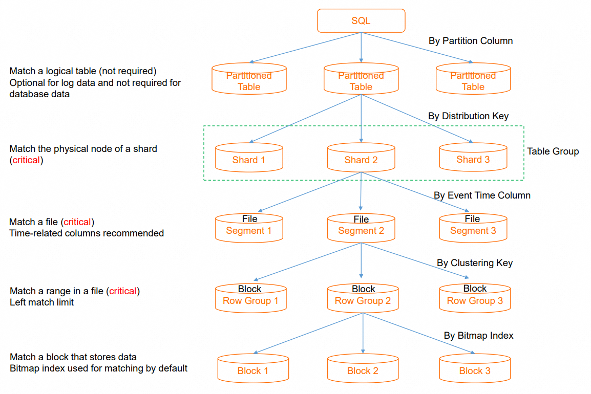
Partition Pruning: When an SQL query is executed on a partitioned table, partition pruning is used to locate the required partition. If a query does not contain a filter condition on the partition key, all partitions must be traversed. This causes excessive I/O scans. A daily granularity for partitions is usually appropriate. This step is skipped for non-partitioned tables.
Shard Pruning: The distribution key (`distribution_key`) is used to quickly locate the data shard that contains the data. This reduces the resource consumption of a single SQL query and provides higher throughput for concurrent SQL queries. If a specific shard cannot be located, the distributed framework schedules all shards to participate in the computation. This increases the degree of parallelism for a single SQL query and uses more resources, which reduces overall concurrency. Some operators that require centralized execution cause additional shuffle overhead. Typically, you should select fields with a balanced distribution, such as order IDs, user IDs, or event IDs, as the distribution key. If multiple tables that need to be joined use the same distribution key, the related data is distributed to the same shard. This enables a Local JOIN for higher join efficiency.
Segment Key Pruning: The segment key (`event_time_column/segment_key`) is used to quickly locate the file that contains the data from multiple files on a single node. This avoids opening unnecessary files. If filtering is not possible, all files on the node must be traversed.
Clustering Key Pruning: The clustering key (`clustering_key`) is used to quickly locate data segments within a single file. This improves the efficiency of range queries and field sorting.
SQL optimization practices
This section uses TPC-H queries as examples to demonstrate how to set Hologres indexes to improve query performance. For more information about TPC-H, see Test plan overview.
TPC-H SQL reference practices
TPC-H Q1 query
TPC-H Q1 aggregates and filters data in specific columns of the `lineitem` table.
l_shipdate <=: Filters the query. An index must be set to support range filtering and accelerate data filtering.
--TPC-H Q1
SELECT
        l_returnflag,
        l_linestatus,
        SUM(l_quantity) AS sum_qty,
        SUM(l_extendedprice) AS sum_base_price,
        SUM(l_extendedprice * (1 - l_discount)) AS sum_disc_price,
        SUM(l_extendedprice * (1 - l_discount) * (1 + l_tax)) AS sum_charge,
        AVG(l_quantity) AS avg_qty,
        AVG(l_extendedprice) AS avg_price,
        AVG(l_discount) AS avg_disc,
        COUNT(*) AS count_order
FROM
        lineitem
WHERE
        l_shipdate <= DATE '1998-12-01' - INTERVAL '120' DAY
GROUP BY
        l_returnflag,
        l_linestatus
ORDER BY
        l_returnflag,
        l_linestatus;
TPC-H Q4 query
TPC-H Q4 mainly performs a join query on the `lineitem` and `orders` tables.
o_orderdate >= DATE '1996-07-01': This is a filter. You can set an index to support range filtering and quickly find the required data.l_orderkey = o_orderkey: This is a join between two tables. You can set the same index for both tables. Performing a Local JOIN is recommended to reduce data shuffle operations during the interaction between the two tables.--TPC-H Q4 Query SELECT o_orderpriority, COUNT(*) AS order_count FROM orders WHERE o_orderdate >= DATE '1996-07-01' AND o_orderdate < DATE '1996-07-01' + INTERVAL '3' MONTH AND EXISTS ( SELECT * FROM lineitem WHERE l_orderkey = o_orderkey AND l_commitdate < l_receiptdate ) GROUP BY o_orderpriority ORDER BY o_orderpriority;
Table creation recommendations
The Q1 and Q4 queries involve the `lineitem` and `orders` tables.
hologres_dataset_tpch_100g.lineitem
Both Q1 and Q4 queries involve the `lineitem` table, but they use different fields and query conditions.
For the Q1 query: The query mainly uses `l_shipdate` for range filtering. The `clustering_key` uses the ordered data within a file to accelerate range filtering. Therefore, you can set `l_shipdate` as the Clustering Key. The `segment_key` (`event_time_column`) is used to maintain order between files. For date fields that are monotonically increasing or decreasing, we recommend that you also set them as the Segment Key. This allows for effective file-level filtering. Therefore, you can also set `l_shipdate` as the Segment Key.
For the Q4 query: The query mainly uses the `l_orderkey` field of the `lineitem` table to join with the `o_orderkey` field of the `orders` table. The `distribution_key` specifies the data distribution policy. The system stores data with the same `distribution_key` value on the same shard. If two tables are in the same table group and their join field is the Distribution Key, records with the same key value from both tables are automatically distributed to the same shard when data is written. When these tables are joined, a Local JOIN is performed on the current node. This avoids data shuffling and redistribution based on the join key at runtime, which can significantly improve execution efficiency. Therefore, set `l_orderkey` as the Distribution Key.
The final table schema for the `lineitem` table is as follows:
BEGIN;
CREATE TABLE hologres_dataset_tpch_100g.lineitem
(
    l_ORDERKEY      BIGINT      NOT NULL,
    L_PARTKEY       INT         NOT NULL,
    L_SUPPKEY       INT         NOT NULL,
    L_LINENUMBER    INT         NOT NULL,
    L_QUANTITY      DECIMAL(15,2) NOT NULL,
    L_EXTENDEDPRICE DECIMAL(15,2) NOT NULL,
    L_DISCOUNT      DECIMAL(15,2) NOT NULL,
    L_TAX           DECIMAL(15,2) NOT NULL,
    L_RETURNFLAG    TEXT        NOT NULL,
    L_LINESTATUS    TEXT        NOT NULL,
    L_SHIPDATE      TIMESTAMPTZ NOT NULL,
    L_COMMITDATE    TIMESTAMPTZ NOT NULL,
    L_RECEIPTDATE   TIMESTAMPTZ NOT NULL,
    L_SHIPINSTRUCT  TEXT        NOT NULL,
    L_SHIPMODE      TEXT        NOT NULL,
    L_COMMENT       TEXT        NOT NULL,
    PRIMARY KEY (L_ORDERKEY,L_LINENUMBER)
)
WITH (
    distribution_key = 'L_ORDERKEY',--Enables Local JOIN for table joins.
    clustering_key = 'L_SHIPDATE',--Accelerates range filtering.
    event_time_column = 'L_SHIPDATE'--Accelerates file pruning.
  );
COMMIT;
hologres_dataset_tpch_100g.orders
In this example, the `orders` table is used in the Q4 query.
Set the `o_orderkey` field of the `orders` table as the Distribution Key to use the Local JOIN capability and improve the efficiency of join queries.
The `o_orderdate` field is mainly used for filtering queries on date fields. You can set it as the Segment Key to accelerate file pruning.
The final table schema for the `orders` table is as follows:
BEGIN;
CREATE TABLE hologres_dataset_tpch_100g.orders
(
    O_ORDERKEY      BIGINT      NOT NULL PRIMARY KEY,
    O_CUSTKEY       INT         NOT NULL,
    O_ORDERSTATUS   TEXT        NOT NULL,
    O_TOTALPRICE    DECIMAL(15,2) NOT NULL,
    O_ORDERDATE     timestamptz NOT NULL,
    O_ORDERPRIORITY TEXT        NOT NULL,
    O_CLERK         TEXT        NOT NULL,
    O_SHIPPRIORITY  INT         NOT NULL,
    O_COMMENT       TEXT        NOT NULL
)
WITH (
    distribution_key = 'O_ORDERKEY',--Enables Local JOIN for table joins.
    event_time_column = 'O_ORDERDATE'--Accelerates file pruning.
  );
COMMIT;
Sample data import
You can use the one-click public dataset import feature in HoloWeb to quickly import the TPC-H 100 GB dataset into your Hologres instance. For more information, see Import public datasets.
Performance test result comparison
After you set the appropriate properties (indexes) for the tables, you can test the performance before and after the optimization.
Test environment
Instance type: 32-core.
Network type: VPC.
Execute the query twice using a PSQL client and record the time of the second execution.
Test conclusion
For filter queries on a single table, setting the filter field as the Clustering Key can significantly accelerate the query.
For queries that join multiple tables, setting the join field as the Distribution Key can significantly improve join efficiency.
Query
Latency with Hologres indexes
Latency without any Hologres indexes
Q1
48.293 ms
59.483 ms
Q4
822.389 ms
3027.957 ms
Appendix
Learn more
Technical principles
To learn about the core principles of Hologres, such as its architecture, storage engine, and compute engine, see Core technologies of Alibaba Cloud's cloud-native real-time data warehouse.
Service activation
To learn how to select an instance type, see Instance management.
For information about RAM user authorization, see Quick Start for RAM user authorization.
Data import
For real-time writes and dimension table queries with Flink, see fully managed Flink.
For real-time synchronization of entire databases, such as MySQL, Oracle, and PolarDB, see Configure a data source (MySQL).
To import OSS data, see Accelerate access to data lakes in OSS based on DLF.
To significantly improve data write and update efficiency, use Fixed Plan. For more information, see Use Fixed Plan to accelerate SQL execution.
Data query
For scenario-based table creation recommendations, see Scenario-based table creation and tuning guide.
When you create a table, you should understand key parameters, such as `distribution_key`, `clustering_key`, `event_time_column`, and `bitmap_index`, and set a reasonable table schema to significantly improve performance. For more information, see CREATE TABLE.
To tune the performance of internal tables, see Best practices: internal table performance tuning.
To accelerate queries on MaxCompute data, see Accelerate queries on MaxCompute data based on foreign tables.
Service monitoring
To troubleshoot active queries and check for locks, see Query management.
To troubleshoot failed or long-running queries, see Get and analyze slow query logs.
For read/write splitting and load isolation, see Deploy primary and secondary instances for read/write splitting (shared storage).
Best practices and use cases
For a collection of best practices and use cases, see Best practices for typical industry scenarios and classic customer use cases.