By He Xu (Tianlie), Chen Haikai (Haikai), Li Yanghua (Yichen), Li Xin (Lixin), and An Bo (Professor from Nanyang Technological University)
The online recommendation service suggests items based on item features and user information. Nowadays, since many users visit e-commerce platforms on their mobile phones, some recommended items are not visible to the users in the first go. To overcome this challenge and remove pseudo exposure in online recommendation scenarios and increase the click-through rate (CTR) of recommended items, we have used the bandit framework for the first time. Incorporating several improvements based on the traditional bandit algorithm has shown good results. This article describes the five key changes implemented to remove pseudo exposure and increase the CTR:
With the popularity of e-commerce platforms, many users use mobile devices to access e-commerce platforms such as Taobao. In recommendation scenarios, a list of items is recommended based on user and item information. Due to the limited screen size, at first glance, a user only sees certain items. To see the remaining items, the user has to swipe through the screen. During this process, the user may tap an item of interest to view its details. After viewing the details, the user may return to the recommendation list to view and tap other items. If no other item is of interest, it is probable that the user will directly exit from the recommendation scenario or Taobao app.
If the user exits from the recommendation scenario before browsing through all the items, this phenomenon is referred to as pseudo exposure. For example, five items are recommended to a user. The user taps the first item to view its details. Then, the user returns to the recommendation list and views the second and third items without tapping either of them. In this case, all we know is that five items were recommended to the user and the user tapped the first item.
Generally, existing findings assume that all the items are viewed by the user, and the items following the third item are considered negative samples. These negative samples with incorrect view information degrade the learning effect.
This article explores how to remove pseudo exposure from online recommendation scenarios and increase the CTR of recommended items. For this purpose, we use the bandit framework, which is a common algorithm for online recommendation scenarios. To use the bandit framework, we must address the following challenges.
This article proposes the innovative contextual multiple-play bandit algorithm to remove these challenges. Let's take a look at the following specific actions:
The multiple-play bandit method is proposed to extend traditional bandit algorithms and recommend multiple arms in each round. The EXP3.M algorithm is extended based on the EXP3 algorithm [7]. The main idea of EXP3.M is to select multiple arms based on EXP3. The Rank Bandit Algorithm (RBA) [18] and Independent Bandit Algorithm (IBA) [10] frameworks are also proposed. In both frameworks, the MAB algorithm is executed at each position to select multiple items.
In the RBA framework, if MAB algorithms at different positions select the same arm, the MAB algorithm at a lower position receives a reward of 0. In the IBA framework, arms selected by the MAB algorithm at a higher position will be deleted from the candidate arms for MAB algorithms at lower positions to prevent repetition. Thompson Sampling is also extended, and theoretical analysis is provided [11].
Recently, multiple-play bandit algorithms are used to maximize the reward sum with limited budgets. [23, 24] However, these algorithms are not context-specific. Therefore, multiple-play bandit algorithms suffer from slow convergence and are unsuitable for large-scale real-life applications.
Pseudo exposure occurs mainly because of the positions of items. Modeling the influence of positions by using a tapping model has been done in some cases. For example, the cascade model [5] has been combined with a multi-armed bandit, combinatorial bandit, contextual bandit, and contextual combinatorial bandit respectively [13, 14, 17, 25].
The combinatorial bandit algorithm recommends a group of items, but only receives the CTR feedback for a set. The cascade model assumes that a user reads recommended documents from top-down until the user finds a relevant document. Wen et al. [22] combine the upper confidence bound (UCB) algorithm with the independent cascade model to present the influence of positions. The cascade model does not support the tapping of diversified items.
Therefore, the PBM is incorporated to [12, 15] estimate the influence of positions on the CTR. Komiama et al. [12] are different from traditional bandit algorithms as they consider the influence of advertisements. Katariya et al. [8] combine the bandit algorithm and the dependent click model, where the latter expands the cascade model to a multiple-click model. All these algorithms assume that a user browses through all items. However, we assume that certain items on mobile apps are not seen by users and use the PBM to estimate the probabilities of seeing items at different positions by users.
This section first describes the problems and the two challenges that mobile e-commerce platforms usually face. Next, we will formulate the contextual multiple-play bandit problem and two CTR evaluation metrics.
With the popularity of mobile phones, more consumers tend to visit e-commerce platforms from mobile clients. Different from web pages, mobile apps suffer from a much smaller display area and therefore display only a few items.
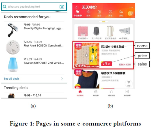
For example, figures 1 (a) and (b) show three and two items, respectively. With this narrow space, it is difficult to learn users' interests, and two challenges must be overcome.
Firstly, the balance between exploration and utilization is very important. Generally, users do not provide additional information about their interests in recommendation scenarios. Therefore, users' browsing and searching records are often regarded as prior knowledge of users. However, items recommended based on prior knowledge are similar to those resulting from search engines. This deviates from the target of exploring users' potential interests in recommendation scenarios. Therefore, the key to this problem is to balance exploration and utilization. This problem is especially important on mobile apps with a limited display area. Exploration is to find users' potential interests without prior knowledge. On the other hand, utilization implies driving users to tap more items and slide through the screen to explore more items. Therefore, we convert the dilemma between exploration and utilization to the multiple-play contextual bandit problem.
Secondly, the obtained data is not perfect. The data do not reflect items that are not viewed by users. Our data is obtained from the "Daily Special Offers" scenario of Taobao, as shown in Figure 1 (b). In this scenario, 12 items are recommended to a user. Due to the narrow display area, only one item is fully visible to the user at first glance. Our data wouldn't reflect whether the user views the remaining items. This phenomenon is called pseudo exposure. To remove pseudo exposure, we need to estimate the probabilities of seeing these items by the user and use these probabilities as the weight of samples. We use the CTR model to estimate the probabilities, which will be described in section 4.
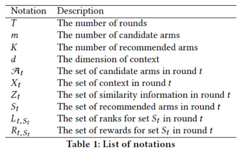
Recommending multiple items based on context information is naturally interpreted as the contextual multiple-play bandit algorithm. Contextual multiple-play bandit algorithm M is executed in round t=1,2,3,...T. In each round T, algorithm M observes the current user u(t), sets A(t) that contains M candidate arms, and sets X(t) that contains vector X(t, a) of each item A in D dimensions. Algorithm M will select a subset S(t) to contain K items based on the observed information. Then, algorithm M will receive the rewards r(t, a) of these items. In addition, sequence L of the items can also be observed by algorithm M. Finally, algorithm M will update the selection policy based on the information (R, X, L). Table 1 lists the main notations.
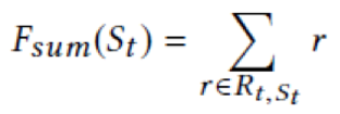
We define two reward equations for recommended item sets:
Sum of taps: The sum of taps on items measures the attractiveness of a recommended item set. At first, we define the reward equation as follows:
Taps on a recommended item set: To prevent a user from exiting, we hope that at least one item in set A(t) of recommended items attract the user and initiates a tap by the user. From this perspective, the reward for the recommended item set is set to 1. If at least one item is tapped, the equation is as follows:

In our recommendation algorithm, the items in a recommended item set are considered arms in a bandit algorithm. If a displayed item is tapped, reward R is set to 1. Otherwise, reward R is set to 0. With this setting, the expected reward is the CTR of items. Therefore, selecting an item to maximize its CTR is equivalent to maximizing the expected reward.
This section proposes the contextual multiple-play bandit algorithm by combining the IBA with a linear reward model. To remove pseudo exposure, we estimate the exposure probabilities at different positions in the linear reward model and use the probabilities as the weight of samples, which is described in section 4.2. To further increase the CTR, we combine the similarity information with the linear reward model, which is described in section 4.3.
Before proposing our algorithm, let's introduce the IBA and LinUCB algorithms.
The IBA is a multiple-play bandit framework that recommends a group of arms. The IBA executes K independent MAB algorithms in sequence. A recommended item set records the items selected by the K MAB algorithms. Items selected by the MAB algorithm at a higher position will be deleted from the candidate items selected by the MAB algorithm at a lower position. This prevents the same item from being selected repeatedly. R(t, S_t) indicates a group of reward vectors. If an item recommended by the K-th MAB algorithm is tapped, the K-th element of the reward vectors is set to 1, but not 0.
The LinUCB algorithm[16] is proposed by Li et al. In the contextual bandit framework, the LinUCB algorithm observes certain context information of items and selects an optimal arm to obtain the highest reward. To use context information, the LinUCB algorithm provides a linear assumption that context information and rewards are linearly related. The LinUCB algorithm is intended to find the optimal parameter to predict rewards based on given context and select an arm with the highest reward.
In the LinUCB algorithm, ridge regression is used to solve the linear regression model. We create a M x D dimensional matrix X. Each row of this matrix contains the context of an element in the recommended item set S(t). R(t) indicates the reward for the recommended item set S(t). When ridge regression is used, the solution is as follows:

We define the following parameters:

The online update equations for the K-th position are as follows:

The UCB for item A(t) is as follows:

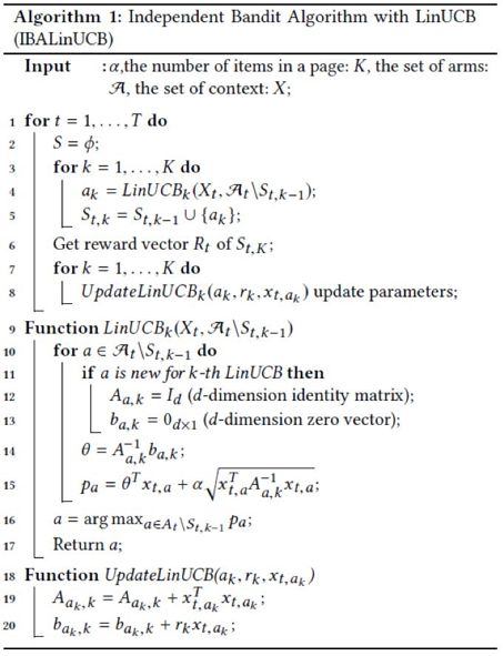
In case, you are wondering where the standard variance of ridge regression is? It is a preset parameter that determines the exploration probability. We propose the IBALinUCB algorithm that combines the IBA and LinUCB. For more information, see algorithm 1. In the fourth row, the K-th LinUCB algorithm is called to select the K-th item. In the fifth row, the selected items are added to a recommended item set. Then, the algorithm obtains the reward for this recommended item set. In the 12th and 13th rows, parameters are initialized. The 15th row provides the formula for calculating the UCB. In the 19th and 20th rows, the parameter update method is defined.
We propose a new algorithm based on algorithm 1 to remove pseudo exposure. Earlier findings show that the CTR greatly depends on positions. Items at top positions are more prone to be tapped [6]. Therefore, we propose the sample weight to estimate the probabilities of seeing the items by users and propose a new linear model. First, let's introduce the CTR model that estimates the sample weight.

In this formula, theta is an unknown vector parameter. W(l) is considered as a constant because it may be learned in advance [15]. To predict R, we combine the weight W(l) with X(a) to develop this new parameter update formulas:
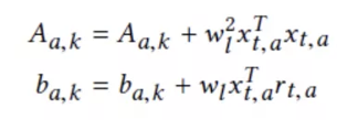
The standard deviation of the K-th position is as follows:

Therefore, the UCB that is used to select items is as follows:

In this formula, alpha is a given constant. The W(k) parameter is constant for each position and is not associated with any items. Therefore, we may ignore this parameter when selecting items. We use the same formula as in the LinUCB algorithm to reduce the calculation workload:

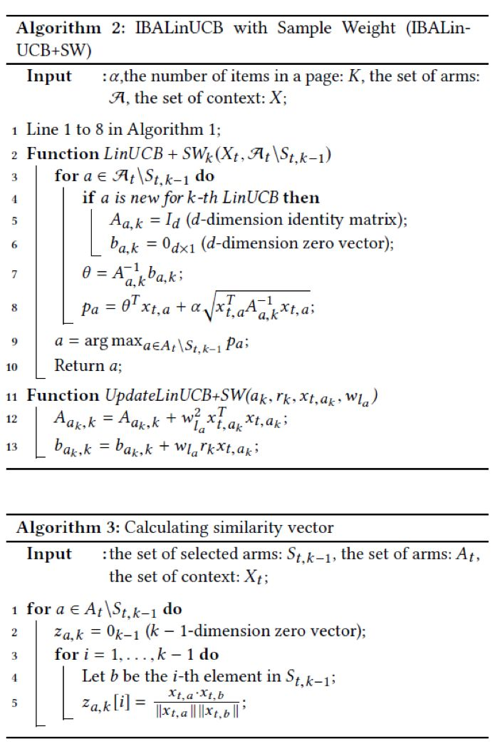
For more information about the IBALinUCB algorithm to which the sample weight is added, see algorithm 2. In the first row, the IBA framework of algorithm 1 is reused. In the second row, the equation for selecting the optimal item at the K-th position is defined. The 11th row shows the method for updating parameters A and b.
Users do not search for specific items in recommendation scenarios. Therefore, the CTR may increase by recommending diversified items. Similarity information is widely used for recommendation, for example, bandit algorithms use similarity information as the Lipschitz condition to prevent items with similar information from obtaining similar rewards [2,9,20]. However, these algorithms recommend one item and receive one reward in each round. We use the cosine similarities to recommend diversified items, which will be described in this section. We adopt a hybrid linear model to use similarity information, as shown in the following formula:

In this formula, we create z(a) as a similarity vector, and beta is an unknown vector parameter that is identical for all items.

After creating the similarity vector, we provide the modified update method based on the HybridUCB[16] algorithm.
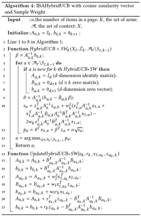
Algorithm 4 provides the IBAHybridUCB algorithm where the similarity information and sample weight are added. In the first row, we ignore the IBA framework, which is displayed in algorithm 1. We define two functions to select items and update parameters. The function in the second row is used to select items based on the UCB. The 14th row provides the equation for updating parameters.
This section analyzes the regret of our algorithm. We analyze the LinUCB+SW algorithm and then provide the regret of the HybridUCB+SW algorithm. Firstly, we define regret in round T based on the reward equation described in section 3. The regret of the sum of rewards is calculated as follows:

In this formula, S(t,*) is the optimal recommended item set in round T. The regret of the rewards of the set is calculated as follows:

In the IBALinUCB+SW algorithm, we prove that the optimal solution selects the first K items with the largest values. For Regret(sum), this point is obvious. For Regret(set), we use sequencing inequality to prove this point. Then, we show that the LinUCB+SW algorithm independently achieves the sublinear regret in the IBA framework.
First, let's restate the regret of the LinUCB algorithm [3] as follows:

Next, obtain the following equation:
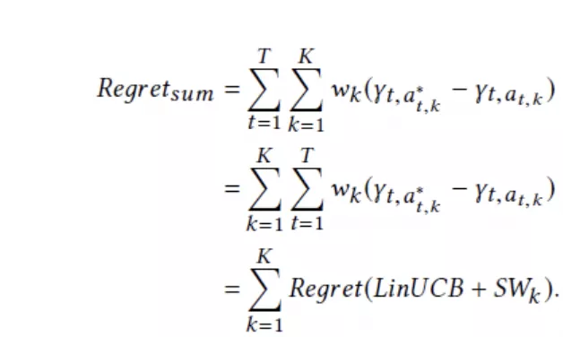
The LinUCB+SW algorithm at the K-th position is determined based on the first K-1 positions, but LinUCB+SW is a random algorithm and the linear model is true for each LinUCB+SW algorithm. Therefore, each LinUCB+SW algorithm obtains the regret in theorem 1.

The proof is as follows:

For the bound of Regret(set), pay attention to the following equation:

The following lemma proves that the K-th algorithm selects the item at the K-th position:
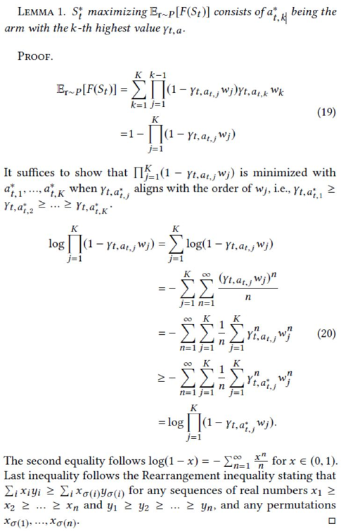
Based on this lemma, the following theorem is obtained:
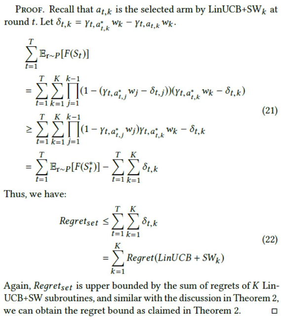
The regret analysis for the LinUCB+SW algorithm also applies to HybridUCB+SW. Although the theoretical analysis of our algorithm is similar to that of the LinUCB algorithm, the test results based on actual data show that our algorithm is much better than LinUCB.
This section describes the testing in detail. Firstly, we define our evaluation metrics. Secondly, we introduce the actual data sets obtained from Taobao and illustrate how to acquire and process the data. We also analyze the existence of pseudo exposure in data. Finally, conduct three tests to evaluate our algorithm. This section compares different algorithms to explore the influence of parameters and the influence of the number of recommended items.
To be consistent with our reward metrics, we propose two evaluation metrics:

We use data provided by Taobao as the source. The data is about a one-day recommendation scenario on Taobao. In this scenario, 12 of 900 items are selected to be displayed to 180,000 users. This scenario has two characteristics. The first is that the number of recommended items is fixed at 12, and mobile Taobao will not recommend new items. The other is that users only see the complete information about the first item and partial information about the second item. As shown in Figure 1 (b), the first item is highlighted with a red box. To view the remaining items, users must scroll through the screen.
The data set contains 180,000 data records. Each data record contains a user ID, the IDs of the 12 items, the context vector of each item, and a tapping vector corresponding to the 12 items. The context vector is a 56-dimensional vector that contains user and item information, such as the items' price and sales, and the purchasing power of users. We remove the data of items that are not tapped because we do not know users' true preferences if they do not view any items.
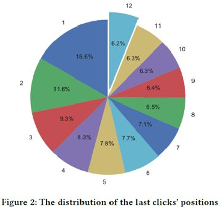
To uncover the problem of pseudo exposure, Figure 2 shows the positions of the last taps. The numbers outside the circle indicate the positions of the last taps. In only 6.2% of records, the last items are tapped. If we assume that pseudo exposure occurs in the items following the positions of the last taps, pseudo exposure occurs in the items in records whose last-tap positions are 1. Based on the weighted sum, about 54% of the samples are affected by pseudo exposure. This percentage is a rough estimate because certain products following the last taps may also be seen by users.
In addition, we use denoising autoencoder [21] to reduce data dimensions. This encoder has four hidden layers and one output layer that contains 56 neural cells. The four hidden layers contain 25, 10, 1, and 25 neural cells respectively. ReLU is the equation for activating the hidden layers. An input vector X is disturbed by a random vector. The input is 0.95x+0.05*noise, where noise is a random vector ranging from 0 to 1. The purpose is to minimize the loss of mean-square error (MSE). We use the output of the second hidden layer as a new context. This extracted context is used in all subsequent tests.
Sample weight is mainly determined by the page structure. Since the page structure is unchanged for a long time, we assume that the influence of positions is a constant [15]. We use the expectation-maximization (EM) algorithm to calculate the same.[4]
We use five contrast algorithms to demonstrate the performance of our algorithm. The first contrast algorithm is a bandit algorithm that does not use context but integrates the PBM. Another two contrast algorithms are widely used contextual bandit algorithms. The fourth contrast algorithm is the LTR algorithm that is used for Taobao. The last contrast algorithm is the algorithm that is introduced in section 4.1.
PBM-UCB[15]: The PBM-UCB algorithm combines the PBM model and the UCB algorithm. The UCB of this algorithm selects the optimal items.

LinUCB-k: This algorithm is directly extended based on the LinUCB algorithm. In each round, this algorithm selects the first K items. After the items are displayed, the algorithm receives rewards for these items and updates parameters based on the LinUCB algorithm.
RBA+LinUCB: The RBA framework [18] executes a bandit algorithm at each position. If the algorithm at the K-th position selects an item that has been selected, the reward received by this position is 0 and the item will be replaced by a random non-repeated item.
LTR: This is an in-depth learning algorithm used for Taobao and is trained by 30 days of data. The output of the neural network is a 56-dimensional vector and is used as the context weight of items. Our data records are sorted by this model. Therefore, we directly select the first K items from the data records for comparison.
IBALinUCB: This algorithm is described in algorithm 1. It is used as a contrast algorithm to reflect the influence of weight.
We conduct three tests and set different K sums to demonstrate the performance of our algorithm. The first test shows the algorithm curves that change with the step when K is 3 and 6 respectively. Then, we reflect on the influence of the changes. In the last test, we demonstrate the final performance of all the algorithms when the number K of recommended items changes. Our IBAhybrid+SW algorithm performs best in most cases.
Figure 3 shows the performance of our algorithm in two metrics. Figures 3 (a) and (c) show the performance of our algorithm when K is 3 and 6 respectively. Figures 3 (b) and (d) show the performance of our algorithm in two evaluation metrics. The IBAhybridUCB+SW algorithm achieves the best performance.
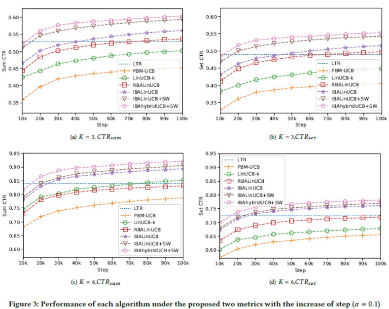
When K is 3, the gap between the other algorithms and the IBAhybridUCB+SW algorithm shown in figures 3 (a) and (b) is larger than that shown in figures 3 (c) and (d). When K is 6, although the performance of our algorithm is 10% higher than that of the LTR algorithm, the gap between the IBAhybridUCB+SW and IBALinUCB algorithms is small. The cause is that when K is large, the sub-optimal algorithm has similar performance to the optimal algorithm. For example, when the recommendation policy is sub-optimal, the optimal item is arranged in the fourth or fifth position and will be displayed when K is 6.
This sub-optimal policy will receive the same reward as the optimal policy. In this case, the algorithm tends to learn a sub-optimal solution, but not an optimal solution. When K is greater, this target is easily achieved than learning the optimal policy. Therefore, contrast algorithms perform better when K is greater. However, our algorithm is less affected by the value of K.
In the second test, we demonstrate the performance of our algorithm when the alpha value is in [0.01,0.6]. Figure 4 shows the test results. In most cases, our algorithm is much better than the other algorithms. At the highest point, our IBAhybridUCB+SW algorithm performs much better than the IBALinUCB+SW algorithm. The following describes our observations. Firstly, due to the lack of exploration, almost all the algorithms perform poorly at that time.
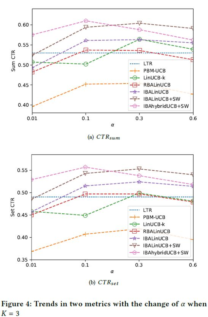
Secondly, almost all the algorithms perform better when the alpha values are 0.1 and 0.3. The reason is that the disturbance caused by variance increases with the increase of the alpha value, and the algorithms tend for exploration. Therefore, the performance of the algorithms degrades.
Thirdly, the IBAhybridUCB+SW algorithm performs better when the alpha value is smaller. This performance is related to the use of similarity information. The IBAhybridUCB+SW algorithm tends to effectively explore and learn the optimal policy based on similarity information. Therefore, this algorithm more efficiently learns data even when the exploration coefficient is small.
We use algorithms to recommend items of different quantities and show the results in Table 2. The LTR algorithm is used as the benchmark algorithm, and the percentage numbers indicate the percentages of CTR increase. Table 2 shows the sum of all the algorithms. A greater CTR indicates that the corresponding algorithm better uses data and learns a better recommendation policy. The number of items in the candidate set is fixed. Therefore, we change the K value to demonstrate the performance of different algorithms at different percentages.
To better understand the results, we use a bar chart for this purpose, as shown in Figure 5. According to our observations, the performance of our algorithm is 10% higher than that of the LTR algorithm. This proves that online recommendation is more suitable for dynamic environments. Among the contrast algorithms, the IBALinUCB algorithm performs better than the other algorithms, and the PBM-UCB algorithm performs poorly due to the lack of context.
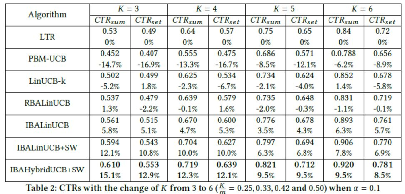
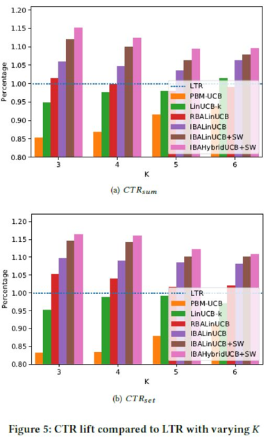
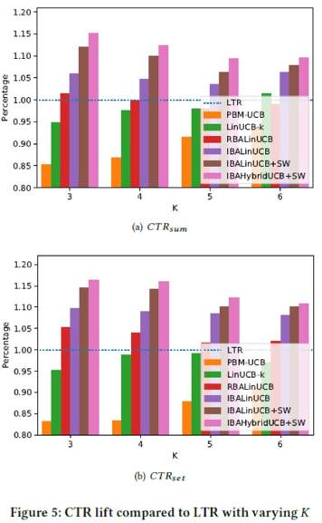
The test results show that our algorithm has better performance when K is 3. The IBAHybridUCB+SW algorithm increases the CTR by 15.1 and 12.9% in the two metrics, respectively. The IBALinUCB+SW algorithm increases the CTR by 12.1% and 10.8% respectively. The results are the same as those in [16]. This article shows that the contextual bandit algorithm has better performance when K is smaller. As mentioned earlier, when K is greater, a sub-optimal policy generates similar results as compared to ones by the optimal policy. Therefore, when K is smaller, the CTR more accurately reflects the performance of algorithms. More importantly, this advantage is critical in actual scenarios because in these scenarios, more than a dozen items are selected from hundreds of items and are recommended to users.
This article focuses on removing pseudo exposure from large-scale mobile e-commerce platforms. Firstly, we depict the online recommendation as the contextual multiple-play bandit algorithm. Secondly, to remove pseudo exposure, we use the PBM model to estimate the probabilities of seeing items by users and use these probabilities as the sample weight. Thirdly, we add similarity information to our linear reward model to recommend items of different types and to increase the CTR. Fourthly, we provide a sublinear theoretical analysis of regret in two metrics. Finally, we conduct three tests by using actual Taobao data to evaluate our algorithm. The test results show that our algorithm significantly increases the CTR compared to a supervised learning algorithm and other bandit algorithms.
References:
[1] Peter Auer. 2002. Using Confidence Bounds for Exploitation-Exploration Trade-offs. Journal of Machine Learning Research 3, Nov (2002), 397-42.
[2] Sébastien Bubeck, Gilles Stoltz, Csaba Szepesvári, and Rémi Munos. 2009. Online Optimization in X-Armed Bandits. In Advances in Neural Information Processing Systems (NIPS). 201-208.
[3] Wei Chu, Lihong Li, Lev Reyzin, and Robert E. Schapire. 2011. Contextual Bandits with Linear Payoff Functions. In Proceedings of the International Conference on Artificial Intelligence and Statistics (AISTATS). 208-214.
[4] Aleksandr Chuklin, Ilya Markov, and Maarten de Rijke. 2015. Click Models for Web Search. Synthesis Lectures on Information Concepts, Retrieval, and Services 7,3 (2015), 1-115.
[5] Nick Craswell, Onno Zoeter, Michael Taylor, and Bill Ramsey. 2008. An experimental comparison of click position-bias models. In Proceedings of International Conference on Web Search and Data Mining (WSDM). 87-94.
[6] Thorsten Joachims, Laura Granka, Bing Pan, Helene Hembrooke, and Geri Gay. Accurately Interpreting Clickthrough Data as Implicit Feedback. In ACM SIGIR Forum, Vol. 51. 4-11.
[7] Sham M Kakade, Shai Shalev-Shwartz, and Ambuj Tewari. 2008. Efficient Bandit Algorithms for Online Multiclass Prediction. In Proceedings of International Conference on Machine Learning (ICML). 440-447.
[8] Sumeet Katariya, Branislav Kveton, Csaba Szepesvari, and ZhengWen. 2016. DCM Bandits: Learning to Rank with Multiple Clicks. In Proceedings of International Conference on Machine Learning (ICML). 1215-1224.
[9] Robert Kleinberg, Aleksandrs Slivkins, and Eli Upfal. 2008. Multi-Armed Bandits in Metric Spaces. In Proceedings of Annual ACM Symposium on Theory of Computing (STOC). 681-690.
[10] Pushmeet Kohli, Mahyar Salek, and Greg Stoddard. 2013. A Fast Bandit Algorithm for Recommendation to Users with Heterogeneous Tastes. In Proceedings of AAAI Conference on Artificial Intelligence (AAAI). 1135-1141.
[11] Junpei Komiyama, Junya Honda, and Hiroshi Nakagawa. 2015. Optimal Regret Analysis of Thompson Sampling in Stochastic Multi-armed Bandit Problem with Multiple Plays. In Proceedings of International Conference on Machine Learning (ICML). 1152-1161.
[12] Junpei Komiyama, Junya Honda, and Akiko Takeda. 2017. Position-based Multiple-play Bandit Problem with Unknown Position Bias. In Advances in Neural Information Processing Systems (NIPS). 4998-5008.
[13] Branislav Kveton, Csaba Szepesvari, ZhengWen, and Azin Ashkan. 2015. Cascading Bandits: Learning to Rank in the Cascade Model. In Proceedings of International Conference on Machine Learning (ICML). 767-776.
[14] Branislav Kveton, Zheng Wen, Azin Ashkan, and Csaba Szepesvári. 2015. Combinatorial Cascading Bandits. In Advances in Neural Information Processing Systems (NIPS). 1450-1458.
[15] Paul Lagrée, Claire Vernade, and Olivier Cappe. 2016. Multiple-Play Bandits in the Position-Based Model. In Advances in Neural Information Processing Systems (NIPS). 1597-1605.
[16] Lihong Li, Wei Chu, John Langford, and Robert E Schapire. 2010. A Contextual-Bandit Approach to Personalized News Article Recommendation. In Proceedings of the International Conference on World Wide Web (WWW). 661-670.
[17] Shuai Li, Baoxiang Wang, Shengyu Zhang, and Wei Chen. 2016. Contextual Combinatorial Cascading Bandits. In Proceedings of International Conference on Machine Learning (ICML). 1245-1253.
[18] Filip Radlinski, Robert Kleinberg, and Thorsten Joachims. 2008. Learning Diverse Rankings with Multi-Armed Bandits. In Proceedings of International Conference on Machine Learning (ICML). 784-791.
[19] Badrul Sarwar, George Karypis, Joseph Konstan, and John Riedl. 2001. Item-Based Collaborative Filtering Recommendation Algorithms. In Proceedings of International Conference on World Wide Web (WWW). 285-295.
[20] Aleksandrs Slivkins. 2014. Contextual Bandits with Similarity Information. Journal of Machine Learning Research 15, 1 (2014), 2533-2568.
[21] Pascal Vincent, Hugo Larochelle, Yoshua Bengio, and Pierre-Antoine Manzagol. Extracting and Composing Robust Features with Denoising Autoencoders. In Proceedings of International Conference on Machine Learning (ICML). 1096-1103.
[22] Zheng Wen, Branislav Kveton, Michal Valko, and Sharan Vaswani. 2016. Online Influence Maximization under Independent Cascade Model with Semi-Bandit Feedback. arXiv preprint arXiv:1605.06593 (2016).
[23] Yingce Xia, Tao Qin, Weidong Ma, Nenghai Yu, and Tie-Yan Liu. 2016. Budgeted Multi-Armed Bandits with Multiple Plays. In Proceedings of International Joint Conference on Artificial Intelligence (IJCAI). 2210-2216.
[24] Datong P Zhou and Claire J Tomlin. 2017. Budget-Constrained Multi-Armed Bandits with Multiple Plays. arXiv preprint arXiv:1711.05928 (2017).
[25] Shi Zong, Hao Ni, Kenny Sung, Nan Rosemary Ke, Zheng Wen, and Branislav Kveton. 2016. Cascading Bandits for Large-Scale Recommendation Problems. In Proceedings of Conference on Uncertainty in Artificial Intelligence (UAI). 835-844.
How to Improve User Participation: The Rise of Interactive Recommendations

2,593 posts | 793 followers
FollowAlibaba Clouder - January 22, 2020
Alibaba Clouder - May 17, 2021
Alibaba Clouder - December 22, 2020
Alibaba Cloud Storage - April 14, 2020
Alibaba Clouder - July 6, 2018
Alibaba Clouder - April 1, 2021

2,593 posts | 793 followers
Follow Platform For AI
A platform that provides enterprise-level data modeling services based on machine learning algorithms to quickly meet your needs for data-driven operations.
Learn More Big Data Consulting for Data Technology Solution
Alibaba Cloud provides big data consulting services to help enterprises leverage advanced data technology.
Learn More Big Data Consulting Services for Retail Solution
Alibaba Cloud experts provide retailers with a lightweight and customized big data consulting service to help you assess your big data maturity and plan your big data journey.
Learn More Epidemic Prediction Solution
This technology can be used to predict the spread of COVID-19 and help decision makers evaluate the impact of various prevention and control measures on the development of the epidemic.
Learn MoreMore Posts by Alibaba Clouder