11.11 The Biggest Deals of the Year. 40% OFF on selected cloud servers with a free 100 GB data transfer! Click here to learn more.
After indexes are created for records in a data table, even if the number of records in the table is huge (hundreds of millions or even billions), it is fast to locate a single record by using the key value query method because the times of comparison is only logN (with 2 as the base) after indexes are created. That is, for one billion data records, the system has to compare data for only 30 times (one billion is approximately equal to 2^30), which takes only tens of milliseconds on a modern computer.
However, if the number of key values to be queried is large (thousands or even tens of thousands) and each key value is searched independently, the read count and comparison count will accumulate to tens or hundreds of thousands, and the latency will increase to dozens of minutes or even hours. In this case, simply using the database indexes for query will be an unbearable experience for users.
The following introduces the combination table function of esProc, which can effectively cope with the preceding problem by searching based on high performance indexes and mass key values. The function is described in the following order:
Note that this article discusses only the implementation on a single machine, and more articles will be published later to further discuss the implementation on a cluster.
The following table with a typical data structure is used as an example:

Create a combination table, and import the source data into the combination table.
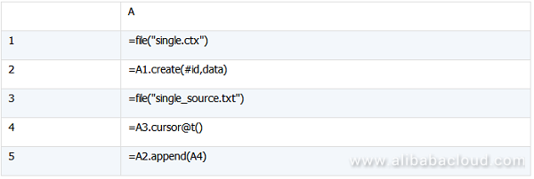
A1: Creates and opens the specified file single.ctx, of which the extension of the combination table is ctx. For detailed definition and use of a combination table, see the esProc tutorials.
A2: Sets the data structure of the combination table to (id, data). The field starting with "#" is called a dimension field, based on which data is sequenced in the combination table. That is, the combination table A2 is ordered by "id". A combination table is stored by column by default.
A3: Opens the data file (assume that the source data is stored by text). In this txt file, the table header and data in the front few rows are shown in the following figure. The source data can also come from other types of data sources, such as databases.

A4: Creates a cursor for the source data, where, "@t" indicates that the first row of the file are the field names.
A5: Appends the records pointed by the cursor A4 to the combination table.
The preceding script assumes that the primary key "id" is already ordered in the original data. If the primary key is not ordered in practice, you must sequence the primary key before creating a combination table. In this case, use the cs.sortx() function for sequencing.
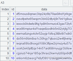
In the esProc designer, you can use three lines of code as shown in the following figure to view the first 10 data records:

A1: Opens the combination table file object with the specified file name.
A2: Directly opens the combination table if no parameter is specified in the f.create() function.
A3: Uses the cursor to access the first 10 data records in A2, as shown in the following figure.
Create an index for the combination table to improve the search performance.

A1: Opens the combination table file object with the specified file name.
A2: Uses the create function without any parameter specified to open the combination table.
A3: Creates an index. In the T.index() function, "id_idx" is the index name, "id" is the dimension, and "data" is the data column. Generally, no data column is needed when you create an index. When searching data using an index, the system accesses the original data table and then finds the data. In this example, however, the data column is also included in the index when the index is being created. In this way, the data column is no longer referenced in the search process. This method consumes more space, but increases the search speed.
When an index is created based on the dimension field, sequencing is not performed again because the combination table is already ordered. If "#" is not used when you start to create a combination table, you need to perform sequencing again when creating the index.
Complete the query by calling the main program and subprogram.
The query subprogram script is search.dfx.
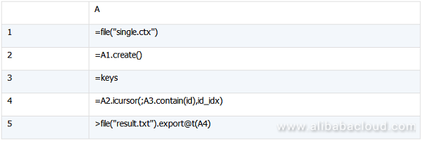
A3: "keys" indicate parameters that are transferred when the following main program is called.
A4: In the icursor() function of the combination table, uses the index "id_idx" and the condition "A3.contain(id)" to filter the combination table. esProc automatically identifies that the condition "A3.contain(id)" can reference the index, sequences the A3 content, and searches data from the front to the back.
A5: Exports the query result of A4 to result.txt. "@t" specifies that the field names are output when the query result is exported.
Main program script:

A1: Obtains the queried key-value sequence from keys.txt. As the result contains only one column, you can use "@i" to return the result as a sequence:
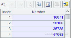
This sequence is the random key-value set to be queried. In this example, keys.txt is used to store the random key values in advance. In practice, you can use other data sources to store the random key values.
A2: Calls the subprogram serach.dfx to transfer the key-value set obtained in A1 to the subprogram.
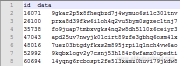
The following figure shows part of the content in result.txt:
Moreover, you can embed esProc in a Java application to provide the flexible and convenient query capability for this application. After embedding esProc, you can access the esProc script like using JDBC to access a database. For more information about coding, see "Calling esProc in Java" in the tutorial.
In this single-field key query example, the data structure is simple. The queried key value field is "id", and the data to be obtained is in a single column. If there are some other columns, for example:
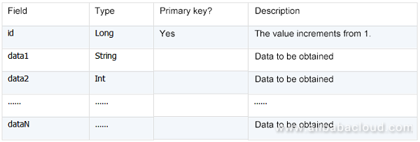
More data column fields should be included in the index creation step. The data column parameters are written as follows:

In the subsequent multi-field key scenario, you need to create multiple index fields, and write the parameters as follows: index(id_idx;id1,id2,…,idN;data1,data2,…,dataN).
A multi-field key refers to a composite primary key. For example,

The two fields, "type" and "id", serve as the composite primary key to determine a record.
Create a combination table
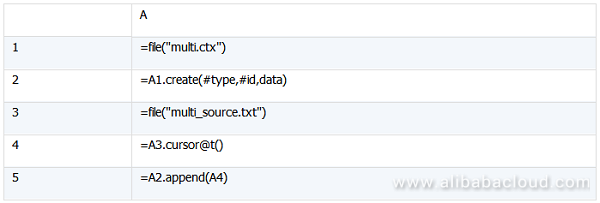
In this example, A2 needs to specify two dimensions, "type" and "id". Other part of the code is the same as that in the single-field key scenario.
Create an index

As there are two dimensions "type" and "id" in this example, you need to include them when creating the index, as shown in A3.
Query data
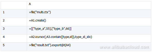
A3 prepares two data records as the key-value sets to be searched, which are 2-tuples composed of "type" and "id". The structures of the two records are as follows:

A4: "A3.contain([type,id])" indicates that data is filtered based on the sequence of 2-tuples. Therefore, parameters in the contain() function must be changed to 2-tuples.
The following shows the content of the result file that is finally exported:

Although the multi-field keys can be directly used, the storage speed and comparison speed are slow if these keys are used. To achieve a high performance, a multiple-field key is often changed into a single-field key by means of merging.
For the data structure in this example, although "type" is a string, it is enumerated. Therefore, "type" can be digitalized and merged with "id" as a new primary key field. As the maximum long-type value is (2^63 - 1), the wide value range can accommodate the result after "id" is merged with the digitalized "type". The new primary key obtained after "type" and "id" are merged is called "nid". Based on the data size, you need to determine how many digits in "nid" can be used to represent "type" and "id", respectively.
For example, the value of "id" contains nine digits, and three digits are sufficient to represent the number of enumerated "type" values. Therefore, "nid" only needs 13 digits. To prevent the case that the first few digits are 0s, you can set the first digit to 1 for alignment purpose. In this way, the composite primary key can be changed into a unique single-field primary key. For the next 12 digits after the first digit "1", the first three digits represent the digitalized "type" and the remaining nine digits represent the original "id".
The code is as follows:
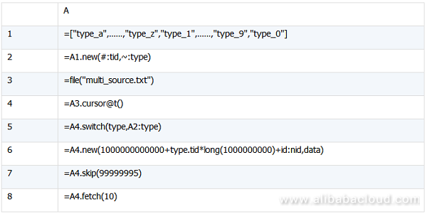
A1: sequence composed of the enumerated "type" values. In practice, the enumerated list may come from a file or a database.
A2: Allocates a "tid" for every "type" value in the enumerated value sequence to prepare for the subsequent merging of the digitalized primary key.
A3 to A6: Obtain data from multi_source.txt and change the enumerated strings in the "type" column into numbers based on the mapping in A2, and merge "type" and "id" into the new primary key "nid".
A7 and A8: Check the data after primary key merging. After skipping the first 99,999,995 records before the cursor A4, you can obtain the following 10 records:
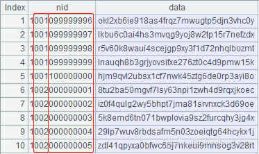
In this way, you can obtain the following data structure of the new single-field key:

Next, proceed using the same method described in the single-field key scenario. Ensure that "nid" must be ordered.
On the basis of the preceding methods, you can use the multi-thread concurrent method to further improve the query performance.
The multi-thread concurrent method means that data is divided into N portions and queried by N threads. However, dividing data into N portions at random may fail to truly improve the performance. This is because a key-value set to be queried is unknown and theoretically it cannot be ensured that the target data can be evenly distributed to every combination table. A better way is to observe the characteristics of the key-value set, on the basis of which data is divided as evenly as possible.
After changing a multi-key field into a single-field key by means of merging in the preceding example, you can use the merged primary key "nid" to perform a modulo operation on 4, store the data with the same remainder in the same combination table, and eventually use four combination tables to load all the existing data. With this file splitting method, you can distribute data to be queried more evenly.
If the key-value data has obvious business characteristics, you can split files based on the fields used in the actual business scenarios, such as the date and department. For example, if you distribute 1,000 records of department A into 10 files evenly, each file has 100 records. When you use multiple threads to query records that belong to department A, each thread extracts these 100 records from the corresponding file.
Let's take a look at actual examples.
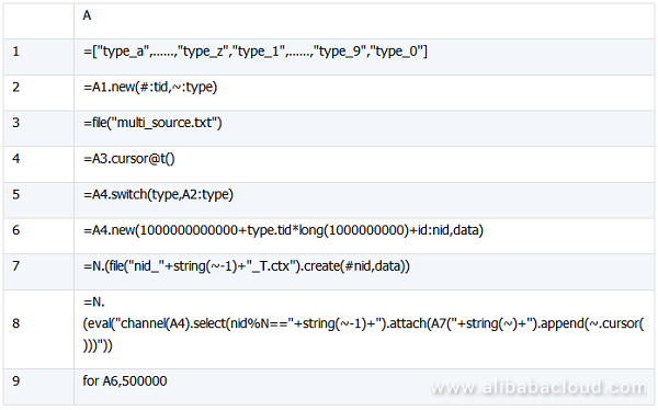
A1 to A6: They are the same as those used in method 2 in the multi-field key scenario.
A7: Uses the loop function to create a combination table named "Key-value name_Remainder of the division of the key value by N_T.ctx". Its structure is also (#nid, data).
A8: Uses the loop function to append the cursor data to N original combination tables. For example, if N is 1, parameters of the eval() function are: channel(A4).select(nid%4==0).attach(A7(1).append(~.cursor())), which indicates the following operations: create a channel for the cursor A4, return the remainder of each record on the channel divided by 4 based on "nid", and filter out records with the remainder 0. "attach" is an attachment operation on the current channel. This operation fetches the original combination table corresponding to the current remainder value, and attaches records that are filtered out from the current channel to A7(1) (that is, the first combination table) as the cursor records.
A9: Uses the FOR loop with the cursor A6 specified to fetch 500,000 records each time until all data in the cursor A6 is fetched.
After execution, four (in this example, N = 4) independent combination tables are output:


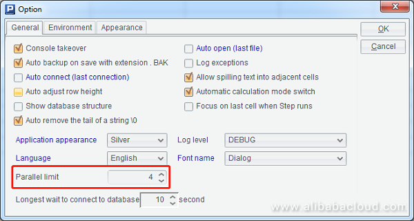
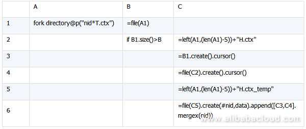
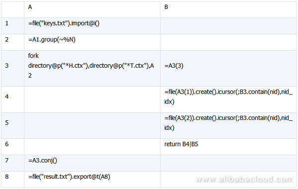
A1: Lists all file names that meet the condition of nidT.ctx, where is the wildcard. Here, "@p" indicates that the file names with the complete path information must be returned. When using the fork() function to execute multiple threads, check whether the parallel limit in the environment is set to an appropriate value. Here, four threads are used, and the corresponding settings in the designer are as follows:
B2: Creates an index file for each combination table in each thread. The final result is as follows:

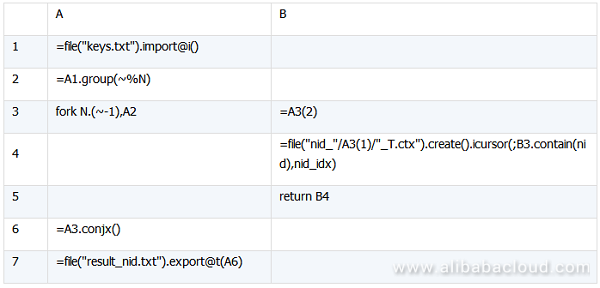
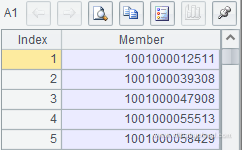
A1: Obtains the key-value sequence to be queried from keys.txt. As there is only one column of the result, "@i" is specified to return the result as a sequence:
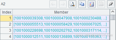
A2: Performs equal value grouping on the A1 sequence based on the remainder of 4:
A3 and B3 to B5: Use the fork() function to perform parallel query on each combination table based on the key values obtained after equal value grouping. Two parameters are specified in the fork() function. The first is the loop function N.(~-1), and the second is A2. In the subsequent B3 and B4, A3(2) and A3(1) are used respectively to fetch the two parameters after the fork() function. In B4, data of the combination table is filtered based on the key-value set in B3. In B5, cursors are returned. As the cursor sequences returned by multiple threads are obtained in A3, CONJX must be used to vertically conjugate multiple cursors in A6.
A6 and A7: Vertically conjugate multiple cursors returned by multiple threads, and export the cursor records to a text file. The first few lines of the text file are as follows:
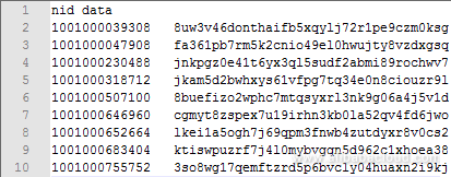
According to the previous descriptions, we have solved the problem of querying mass random key values in a large amount of data. However, we cannot assume that data never changes. Appending of new data is inevitable especially for big data. Three cases may arise when you append new data to the original combination tables: appending of ordered key values, appending of unordered key values, and appending of a large amount of data.
If key values are ordered in a single file, the code for appending data is as follows:
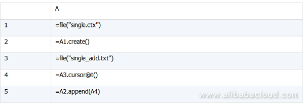
A1: single.ctx is the existing combination table file with the structure of (#id,data), where "id" is a self-increasing key value.
A3 to A5: The structure of the new data file is the same as that of the existing file. After "id" of the new data file is added to the original combination table, "id" is still ordered for all the data. In this case, the data can be directly appended to the original combination table, and the original combination table automatically updates indexes.
If data is split into multiple files according to the multi-thread method, the code is as follows:
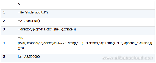
A1 and A2: Use the cursor to obtain the new data.
A3: Lists in sequence the existing N combination table files that meet the wildcard string "id*T.ctx".
A4 and A5: They are the same as the code in the previous method.
The code for appending single-field key values to a single file is as follows:
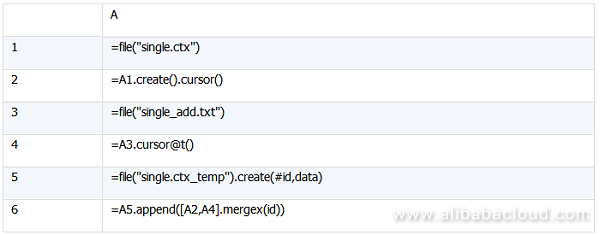
A2: Uses the cursor to open the existing combination table.
A4: Uses the cursor to obtain the new data.
A5: Creates a combination table file.
A6: Stores the result in the new combination table after the data of the existing combination table is merged with the new data. To use cs.mergex(x) for data merging, the cursor sequence (CS) must be ordered by x. That is, both the combination table file A1 and the new data file A3 are ordered by "id". If the CS is not ordered by x, the merging result is also unordered even if the program does not report an error.
After executing this section of the code, clear the old combination table and old indexes and create indexes for the new combination table:

The first three lines are file operations. For more information, see the description about movefile in "Function Reference". A4 is used to create indexes for the combination table, and is already explained earlier.
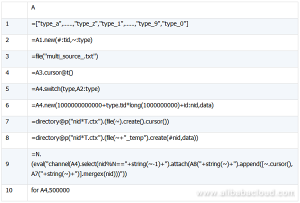
The following takes the data structure (nid, data) after the multi-field key is changed to a single-field key as an example to describe how to append data to multiple files. The code is as follows:
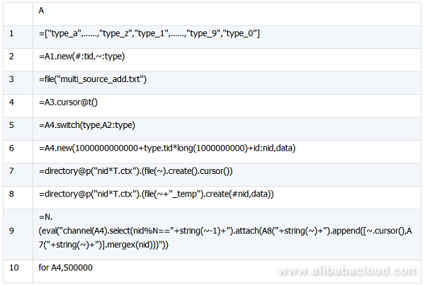
A3: multi_source_add.txt is the new data source.
A7: Assuming that old combination tables already exist, lists the file names of the old combination tables, obtains the cursors of the combination tables in sequence, and returns the result as a sequence.
A8: Creates a combination table file, which is used to store the data of the old combination table and the new data. "_temp" is added at the end of the old file name for differentiation purpose.
A9: Uses the channel for the new data, merges the N cursor records on the channel with the cursor records in N old combination tables, and appends the data to N new combination tables. Detailed explanations are already provided above.
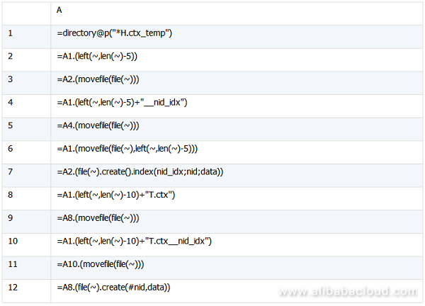
After executing this section of the code, you also need to clear the old combination tables and old indexes and create indexes for the new combination tables:
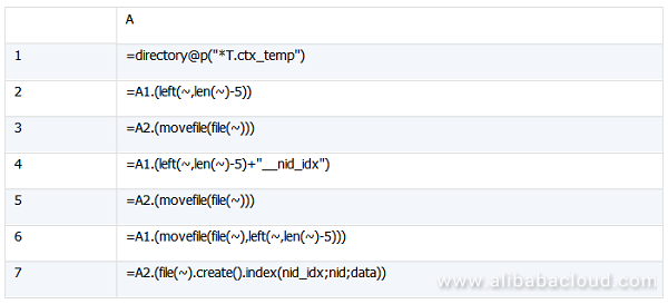
The code mainly contains the loop functions and simple file operations. For more information about functions, see the descriptions in "Files". The last line is used to create indexes, which has been explained above.
With continuous increase of new data, a longer time and a higher cost are required for merging the appended data and full historical data. In this case, you need to split each combination table file into two files. One stores the appended data that is accumulated in the latest period of time and is called new-portion combination table file, and the other stores the historical data and is called old-portion combination table file. New data is still appended according to the method described earlier, except that the operations are performed only on the new-portion combination table file. When the size of the new-portion combination table file exceeds the threshold (for example, 100 GB), this file is merged with the old-portion combination table file. This method not only reduces the time and cost required for merging, but also reduces the disk loss.
Again, by taking the data structure (nid,data) as an example, let's review the entire code:
First, define the new-portion and old-portion combination table files. The naming rules are as follows:
New-portion combination table file: Key value name Remainder of the key value divided by N_T.ctx; Old-portion combination table file: Key value name Remainder of the key value divided by N_H.ctx.

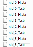
N is equal to 4. The new-portion and old-portion combination table files generated for the preceding four files are as follows:

By now, based on the six esProc script files provided in this article, you can append a large amount of data and query massive random key values on a single machine by properly using the third-party task scheduling tool.
When Databases Meet FPGA – Achieving 1 Million TPS with X-DB Heterogeneous Computing

2,593 posts | 793 followers
Followdigoal - April 12, 2019
ApsaraDB - December 26, 2023
Alibaba EMR - May 20, 2022
Alibaba Clouder - July 5, 2019
ApsaraDB - November 17, 2020
ApsaraDB - October 21, 2024

2,593 posts | 793 followers
Follow Alibaba Cloud for Manufacturing
Gain an industrial edge with Alibaba Cloud best practices
Learn More Key Management Service
Create, delete and manage encryption keys with Alibaba Cloud Key Management Service
Learn More Cloud Hardware Security Module (HSM)
Industry-standard hardware security modules (HSMs) deployed on Alibaba Cloud.
Learn More Database for FinTech Solution
Leverage cloud-native database solutions dedicated for FinTech.
Learn MoreMore Posts by Alibaba Clouder