I once attended a RAG demo for a customer. Each question produced a plausible answer from the documents, and the people around the table nodded along.
Then someone asked, "So how accurate is it?"
The room went quiet. I had no number to give them. We had tried several questions and the answers looked good, but that was not enough to call the system accurate. In a meeting where the decision is whether to take it to production, "it usually works" is not evidence.
Only after experiencing that silence did I realize what was missing. I did not need a better explanation. I needed a way to measure accuracy.
To turn accuracy into a number you can say out loud, you first have to settle three settings and find a way to measure the result:
So let me answer the meeting-room question up front, because it is the most important number in this post. The same model, asked the same 30 questions with no retrieval at all, answers only 2 of them correctly. With retrieval, it answers up to 29. That gap, not the model, is what a RAG pipeline actually produces, and measuring it is the point of everything below.
These are not questions with one universal answer. They depend on your corpus, your queries, and your quality bar. The honest way to answer them is not to pick a number from a blog post. It is to measure them on your own system.
So this post takes a different approach. Instead of recommending settings, I built an enterprise-knowledge RAG entirely on managed Alibaba Cloud services: Model Studio for the models and AnalyticDB for PostgreSQL for vector search. I then ran a full factorial evaluation of 3 chunk sizes × 3 top-k values × rerank on/off = 18 configurations, scoring each one on retrieval recall, answer correctness, groundedness, and refusal. Every number below is measured, not claimed.
Rather than just describing the idea, this post walks through the whole process: building a credible corpus, setting up the vector index, creating a reusable evaluation harness, judging at half price with the Batch API, and analyzing the measured results. The system was built and verified in a real environment. At the end I hand over the harness and an interactive playground you can reuse.
One clarification up front: "accuracy" here is measured against a fixed golden QA set by an LLM-as-judge, not graded by a human. That makes it cheap and reproducible, but treat it as a comparative instrument for choosing between configurations, not as absolute truth. See the Limitations section.
The system has three lanes: ingest, query, and evaluate. The point of the diagram is that evaluate is not a separate track running beside query. It wraps the query pipeline. The matrix drives it once per configuration (18 times) and scores every run.
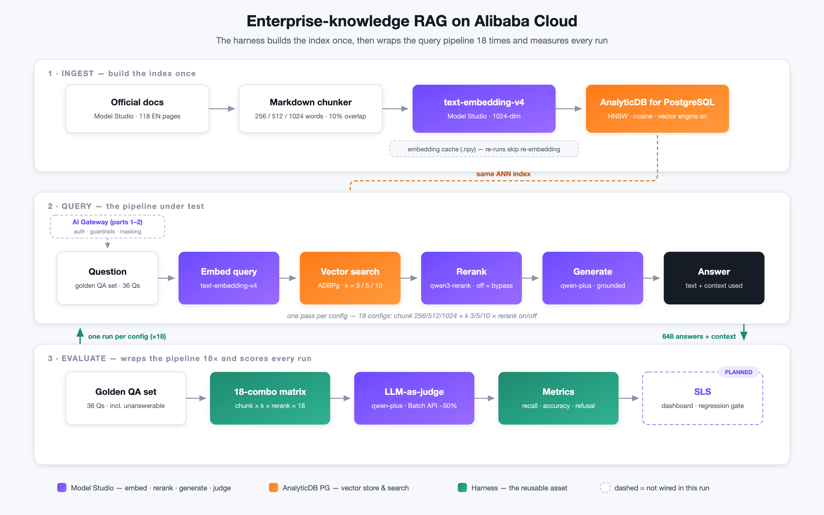
text-embedding-v4, and loaded into an ANN index on AnalyticDB for PostgreSQL. An embedding cache means re-runs skip re-embedding.qwen3-rerank (the rerank on/off branch is one of the experimental axes), then answered by qwen-plus with a strict grounded prompt.The key point: the pipeline and the measurement are one artifact. The same harness that builds the index also scores it, so every time you change a setting you get a comparable number back. That is what turns "RAG tuning" from guesswork into a regression test.
A RAG benchmark is only as credible as its knowledge base. Point it at three hand-written files and you are really testing whether it can find the only relevant document. That is trivial and not what production looks like.
So I used a real corpus. I scraped the complete English (international) Model Studio documentation: 118 pages and about 4.3 million characters. I then converted it to clean Markdown while preserving tables and code fences. This matters for two reasons.
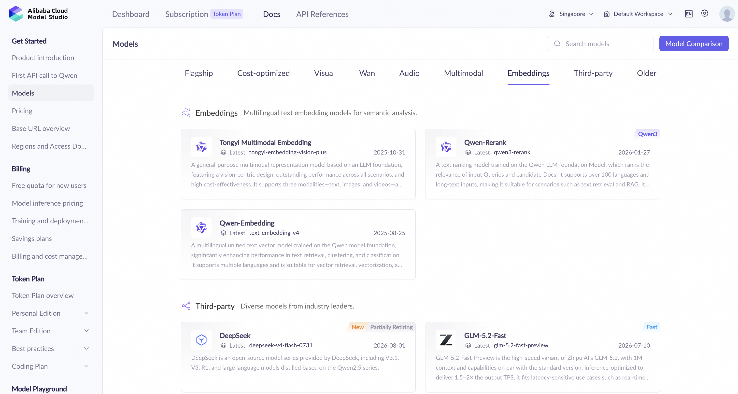
All the models come from Model Studio's catalog. For this build: text-embedding-v4 for embedding, qwen3-rerank for reranking, and qwen-plus for both answer generation and judging.
Why the corpus choice matters for the numbers: groundedness scores are high partly because this corpus is clean and authoritative. Messier enterprise documents, including scans, mixed languages, and stale pages, will be harder. That is a reason to keep the harness and re-measure, not to assume these numbers transfer.
I chunked the same corpus three ways: 256, 512, and 1024 words with 10% overlap. This produced 3,087 / 1,397 / 676 chunks respectively. The chunker is Markdown-aware and, importantly, splits oversized blocks (huge Markdown tables) so no single chunk blows past the embedding model's token limit. That last point cost me an InternalError on the first run. A 40-column pricing table became one giant "paragraph" until I added the split.
Each chunk is embedded with text-embedding-v4 at 1024 dimensions.
From my implementation: I added an on-disk embedding cache keyed by a content hash of the chunks. Every time you re-run the matrix you would otherwise re-embed thousands of chunks and pay for them again. With the cache, re-runs load vectors from disk. For an eval you run on every change, this is the difference between a cheap regression gate and an expensive one.
The vector store is AnalyticDB for PostgreSQL 7.0 in Elastic Storage Mode, created with Vector Engine Optimization enabled. This is a toggle at instance creation, so verify that it shows Enabled before you build the index.
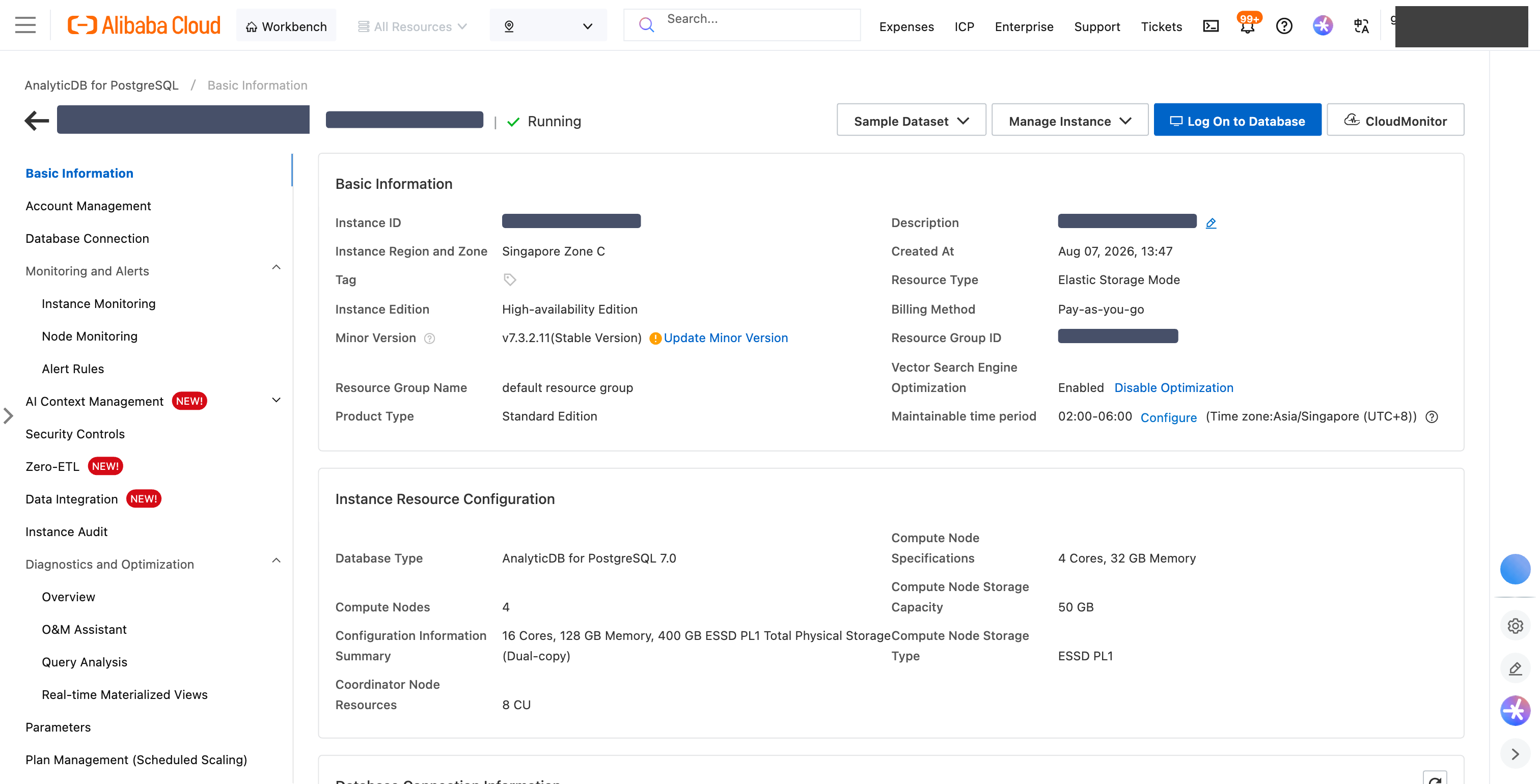
Example configuration: an AnalyticDB for PostgreSQL instance in the console. If you follow along, confirm Vector Engine Optimization shows Enabled before you build the index.
You may also spot Enable RAG Service in that connection panel. AnalyticDB for PostgreSQL ships with a built-in RAG capability. It is a fast way to stand up a retrieval pipeline, and if a working endpoint is all you need, you should absolutely consider it. The reason I did not use it here is the point of this post: the built-in service does not expose chunk size, top-k, or the reranker as knobs you can vary and measure. This article is about measuring those settings, so I assembled the pipeline myself and made every stage, from chunking and embedding through retrieval, reranking, and generation, an explicit and measurable variable. Think of the built-in service as the quick path to a working RAG, and the harness in this post as the tool for when you need to know which settings actually matter.
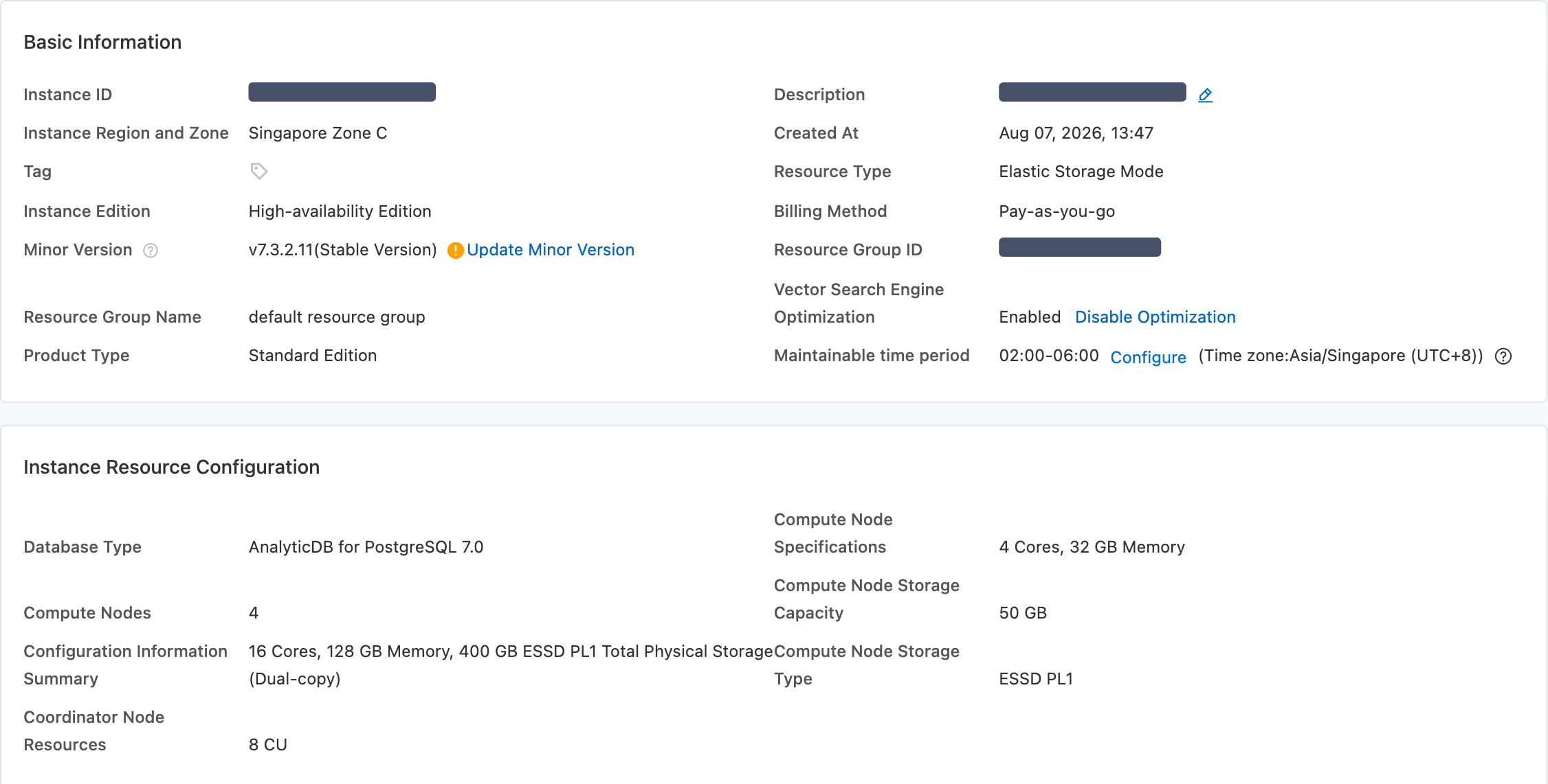
Instance detail: note Vector Search Engine Optimization: Enabled at the bottom. This is what makes the ANN index fast.
The schema is a single chunks table with a vector(1024) column and an ANN index using cosine distance.
CREATE TABLE chunks (
    chunk_id  text,
    doc_id    text,
    chunk_seq int,
    content   text,
    embedding vector(1024)
) DISTRIBUTED BY (chunk_id);

CREATE INDEX chunks_vec_idx ON chunks USING ann(embedding)
WITH (dim=1024, distancemeasure=cosine, hnsw_m=16, pq_segments=64);
Retrieval is an ANN nearest-neighbor search with <=>, returning the top-k by cosine similarity.
SELECT chunk_id, doc_id, content,
       cosine_similarity(embedding, '<query_vector>'::vector) AS score
FROM chunks
ORDER BY embedding <=> '<query_vector>'::vector
LIMIT 10;
From my testing: the upsert is the bottleneck, not the search. My first loader inserted rows one at a time. Pushing ~3,000 vector rows across single-row
INSERTs to a remote instance took many minutes and looked hung. Switching to a batched multi-row insert (psycopg2.extras.execute_values) loaded 3,087 rows in about 6 seconds. If your ingest feels stuck, batch the inserts before you blame the database.
The pipeline is disposable. The harness is the asset. It lives in a small Python package and does five things: chunk, embed, index/retrieve, generate, and judge. But the heart of it is the golden QA set and the metric definitions.
I hand-wrote 36 questions, deliberately mixed so the eval measures different failure modes:
| Type | Count | What it tests |
|---|---|---|
| Single-hop | 12 | One fact, one document |
| Multi-hop | 10 | Must combine two documents |
| Paraphrase | 8 | Same facts, asked casually to test robustness |
| Unanswerable | 6 | Not in the docs, so it must refuse rather than invent |
Each answerable question lists its golden source document(s), which makes recall@k deterministic: did a retrieved chunk actually come from a document that contains the answer?
The unanswerable set is the one most people skip, and it is the most valuable. Questions like "What is the guaranteed uptime SLA percentage?" have no answer in the corpus. A production RAG that confidently invents one is worse than one that says "not found." These six questions measure exactly that.
correct vs partial/incorrect).The harness loops over every combination, retrieves (and optionally reranks), generates, and writes one row per (combo, question).
# Production run against AnalyticDB for PostgreSQL
export DASHSCOPE_API_KEY=sk-xxx
export ADBPG_HOST=... ADBPG_USER=... ADBPG_PASSWORD=... ADBPG_DB=rag_eval
python run_matrix.py --retriever adbpg

# Dev loop without a database (numpy cosine baseline)
python run_matrix.py --retriever local
That produces 18 combos × 36 questions = 648 generated answers to judge.
If you want to reproduce this, here is the actual shape of the project. The whole thing is a small Python package. There is no framework.
harness/
  config.py            models, endpoints, matrix dims, ADBPG connection, .env loader
  chunker.py           markdown-aware chunking with overlap (splits oversized tables)
  embedder.py          text-embedding-v4 + on-disk embedding cache
  reranker.py          qwen3-rerank (DashScope native rerank API)
  retriever_local.py   numpy cosine baseline (develop without a database)
  retriever_adbpg.py   AnalyticDB ANN index (cosine), batched upsert
  generator.py         qwen-plus answer generation with a strict grounded prompt
  judge.py             LLM-as-judge prompt + output parser
  run_matrix.py        runs the full matrix, writes per-combo JSONL
  batch_judge.py       judge via Batch API (50% cost), merges results
  aggregate.py         judged results -> per-combo recall/accuracy/groundedness
  make_charts.py       renders the charts used in this post
  gen_demo.py          builds the interactive playground (demo.html)
The data flow is a straight line: corpus/ → chunks → embeddings → ADBPG index → retrieve → (rerank) → generate → judge → metrics. Every stage is its own module, so you can swap one piece, such as the generator model or the retriever, without touching the rest.
https://dashscope-intl.aliyuncs.com/compatible-mode/v1) if you are in Singapore.# requirements.txt
openai
psycopg2-binary
numpy
matplotlib
scikit-learn# harness/.env (chmod 600)
DASHSCOPE_API_KEY=sk-xxxxxxxx
ADBPG_HOST=gp-xxxx.gpdb.singapore.rds.aliyuncs.com
ADBPG_PORT=5432
ADBPG_DB=rag_eval
ADBPG_USER=rag_eval
ADBPG_PASSWORD=********corpus/ (Markdown), and the golden QA set in golden_set.jsonl (each answerable row carries its source_docs).run_matrix.py (retrieve + generate), batch_judge.py (score at half price), aggregate.py (report). The optional make_charts.py and gen_demo.py produce the visuals.cd harness
python run_matrix.py --retriever adbpg
python batch_judge.py --dir results --pattern 'run_*.jsonl'
python aggregate.py --file results/results_judged.jsonlThat is the entire system. The managed services handle the heavy lifting, including embedding, ANN search, and judging. The harness just orchestrates and measures.
The configuration numbers above are the result, but the process that got there is the reusable part. A few principles, and the specific mistakes that shaped the build:
Build local first, promote to the managed service last. The harness has two retrievers for a reason. I developed against retriever_local.py, a NumPy cosine baseline that needs no database, to validate chunking, the golden set, and the generation prompt cheaply and quickly. Only once the loop was sound did I point it at AnalyticDB. Keep the expensive path for last. You will iterate on it far less.
Measure retrieval and generation separately. recall@k is deterministic and isolates retrieval. The judge scores generation. When a number is bad, this split tells you which stage to fix. Low recall with good accuracy means the retriever is missing the document. Good recall with low accuracy means the generator is fumbling the context. Without the split you are just guessing.
Iterate on real failures. Every "optimization" in the final harness came from hitting an actual wall, not from anticipation:
InternalError. Fix: the chunker now splits any block larger than the chunk size before packing.INSERT at a time over a WAN link took many minutes. Fix: use a batched multi-row insert. It loaded 3,087 rows in about 6 seconds.source_docs, and re-verify the unanswerable questions stay unanswerable.Treat the evaluation as a regression gate. The golden set lives in version control alongside the harness. Any change, whether it involves new documents, a new model, or a new chunk size, gets re-run and diffed against the previous metrics. That turns "did I make it better?" from a feeling into a number.
Scoring 648 answers with a real-time LLM is the most expensive part of the loop. It is also the part you re-run every time the corpus or a setting changes. So I packaged all 648 judge calls into a single Model Studio Batch API job, which runs at 50% of real-time pricing within a 24-hour window.
The same qwen-plus judge, temperature=0, and prompt run at half the cost with no added code complexity. It is just the OpenAI-compatible /v1/batches endpoint: build a JSONL of chat-completion requests, upload it, poll, and merge the outputs back.
# Judge all 648 answers at 50% cost, merge into results_judged.jsonl
python batch_judge.py --dir results --pattern 'run_*.jsonl'

# Aggregate into per-combo metrics
python aggregate.py --file results/results_judged.jsonl
For an evaluation you intend to run repeatedly, the Batch API is what makes "re-measure on every change" affordable.
Two reading notes before the numbers, because they matter more than any single figure.
Resolution: read the two tables differently. The per-combination numbers (the table in 8-3) are each computed over 30 answerable questions, so one question is worth 3.3 points. A gap of less than ~10 points between two individual combos represents only one or two questions and sits inside the judge's run-to-run variance. Read it as noise, not as a ranking. The marginal means in 8-1 are different. Each one averages six configurations, or 180 answerable question-instances, so they are far more stable. That is exactly why the conclusions below are drawn from the marginal means, not from individual cells.
The control: can the model already answer these without retrieval? This decides whether the numbers mean anything. The corpus is Model Studio's own documentation, and the generator and judge are both qwen-plus, a model that plausibly saw these pages during pretraining. If it already knows the answers, the accuracy below could be memorization, not retrieval. So I ran the same 36 questions past qwen-plus with no retrieved context at all, using a neutral prompt and the same judging rubric:
| Closed-book (no retrieval) | RAG, best config | |
|---|---|---|
| Answerable accuracy | 0.067 (2/30) | 0.967 |
| Unanswerable refusal | 0.000 | 1.000 |
Without retrieval, qwen-plus gets only 2 of 30 past the judge, and both are hollow wins. One produced the right number while citing the wrong vendor's documentation. The other simply declined, and the judge's "correct" there reflects leniency rather than knowledge. Substantively, closed-book recall is effectively zero. On parametric knowledge alone the model even confused Alibaba Cloud Model Studio with a different vendor's product of the same name. So the accuracy below is retrieval doing the work, not the model remembering the docs. In closed-book mode, it also fails to refuse the unanswerable questions. The grounded prompt plus retrieved context produces the 1.0 refusal rate.
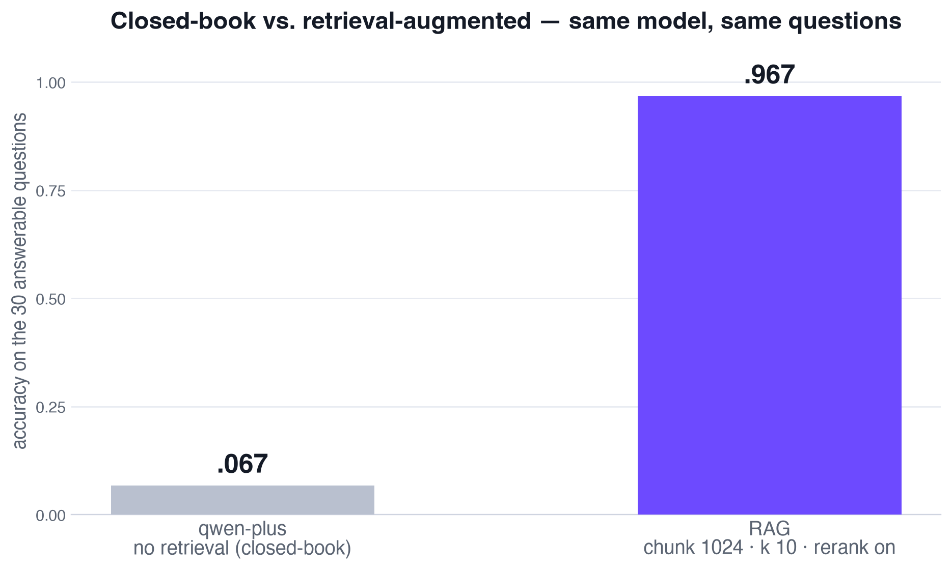
Same model, same 30 answerable questions: without retrieval only 2 of 30 get past the judge. Add retrieval and it is 29 of 30.
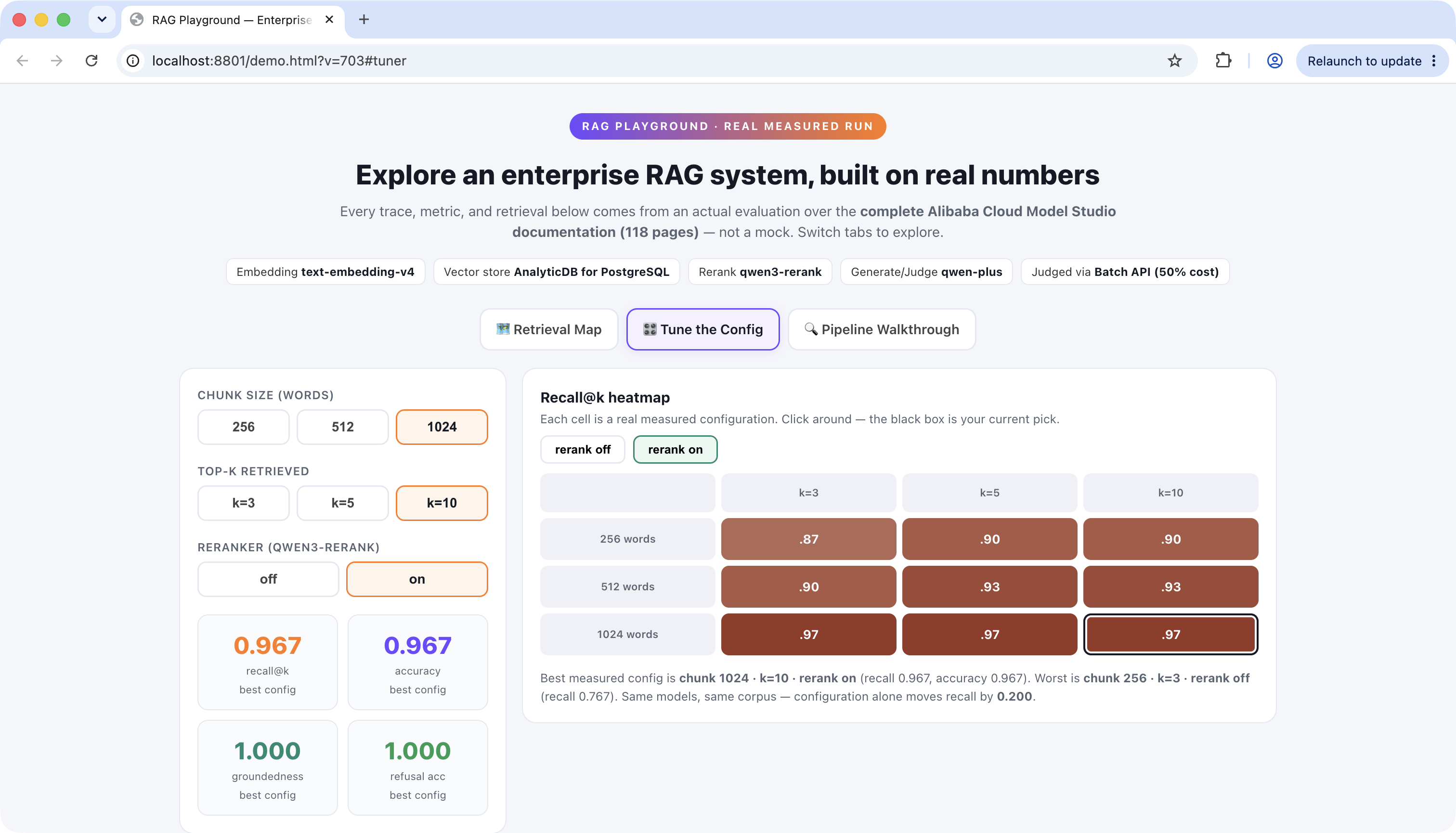
Best single configuration: chunk 1024 · top-k 10 · rerank on:
| Metric | Score |
|---|---|
| recall@10 | 0.967 |
| accuracy | 0.967 |
| groundedness | 1.000 |
| refusal accuracy | 1.000 |
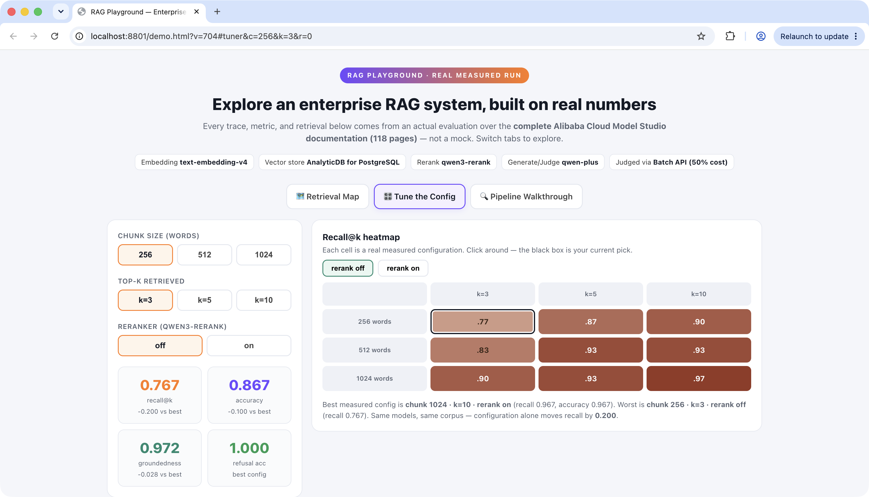
Across all 18 configurations, recall ranged from 0.767 to 0.967 and accuracy from 0.833 to 0.967. Groundedness stayed above 0.94 everywhere, and refusal accuracy was 1.0 in every configuration. The grounded prompt never let the model invent an answer to an unanswerable question.
Chunk size is the biggest lever.
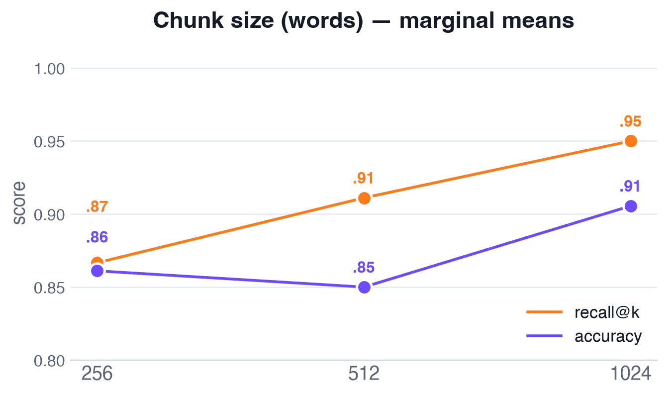
Going 256 → 512 → 1024 words lifted recall from 0.867 → 0.911 → 0.950 and accuracy from 0.861 → 0.850 → 0.906. Larger chunks keep more surrounding context intact, so the retriever hands the generator complete, self-contained passages instead of fragments. The small accuracy dip at 512 is within judge run-to-run variance. The 256→1024 trend is unambiguous.
One fairness caveat on that recall comparison: at a fixed k, larger chunks retrieve a larger fraction of the corpus per query. At k=10, that is about 1.5% of the 676 chunk-1024 index but only ~0.3% of the 3,087 chunk-256 index. So part of the chunk-size recall gain is a token-budget artifact, not purely a chunking effect. A strict comparison would hold the retrieved-token budget constant by raising k for smaller chunks until each combo pulls back roughly the same number of tokens. The direction of the finding still holds because larger chunks help here. However, this fixed-k comparison somewhat overstates the size of the chunk-size advantage.
Top-k has a clear but smaller effect.
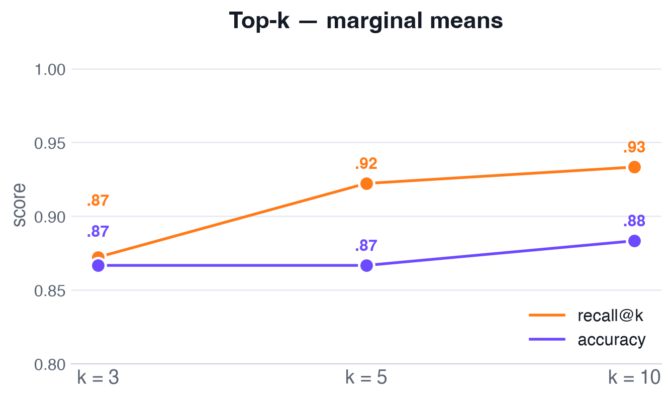
Recall climbs 0.872 (k=3) → 0.922 (k=5) → 0.933 (k=10). Retrieving more candidates gives the reranker and generator more to work with. The gain is already flattening by k=10. I did not measure beyond 10, but past that flattening point extra candidates are more likely to add latency and cost than recall.
Rerank buys recall, roughly breaks even on accuracy.
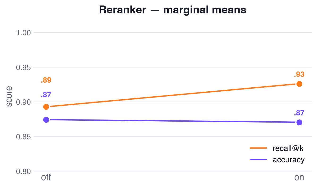
Turning the reranker on lifted recall from 0.893 → 0.926. Accuracy was essentially flat (0.874 → 0.870) and groundedness dipped slightly (0.978 → 0.969). So the reranker's job here is to promote the right document into the context window. Whether you enable it is a recall-vs-latency/cost trade.
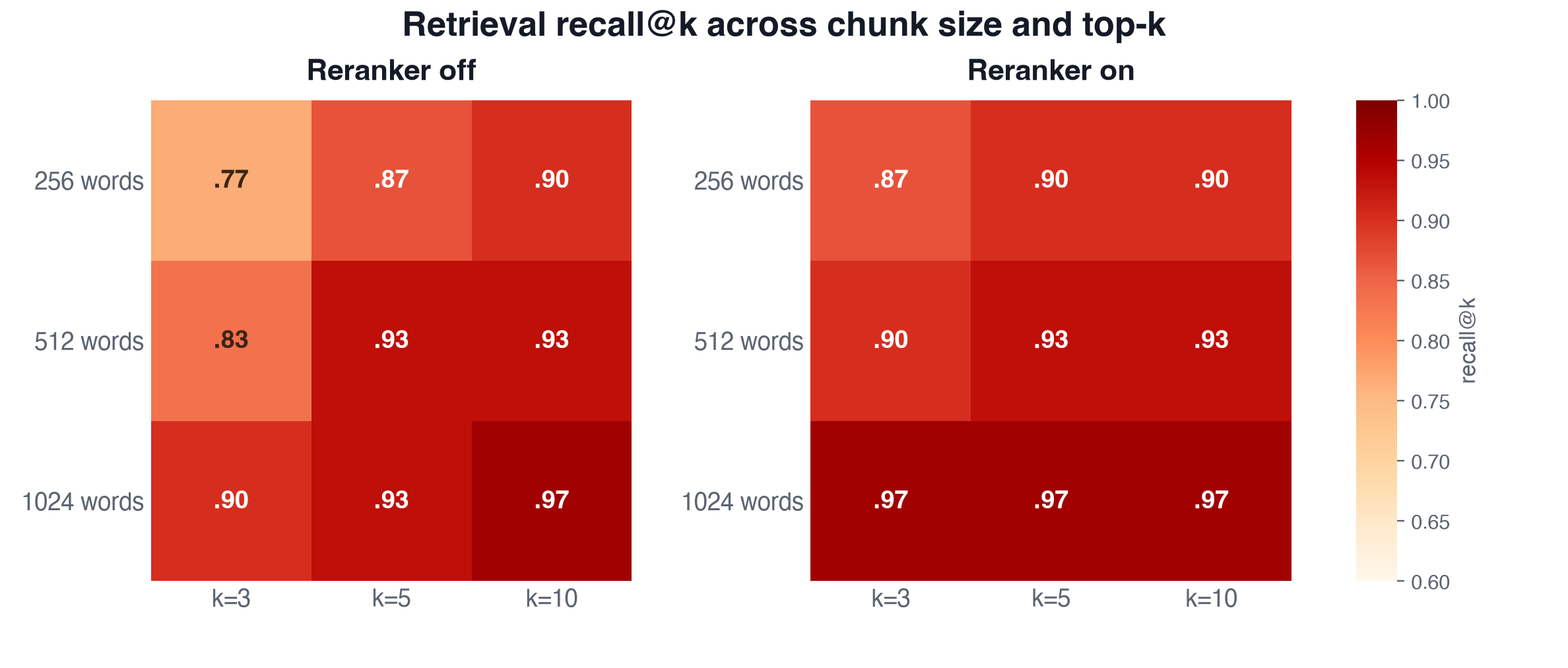
Two things jump out. First, recall is non-decreasing as you move toward larger chunks and higher k. It rises or holds and never drops. The rerank-on 1024 row is flat at 0.97, and the 512 row flattens from k=5. Second, reranking flattens the curve. With it on, even the small-chunk and low-k corners reach ~0.87, and the whole 1024 row saturates at 0.97. If you can only afford one knob, choose chunk size. The reranker is what rescues a mediocre configuration.
| Combo | recall | accuracy | ground | refusal | p95 latency | cost/query |
|---|---|---|---|---|---|---|
| c256_k3_r0 | 0.767 | 0.867 | 0.972 | 1.0 | 4.4s | $0.0005 |
| c256_k3_r1 | 0.867 | 0.833 | 0.944 | 1.0 | 4.5s | $0.0010 |
| c256_k5_r0 | 0.867 | 0.867 | 1.000 | 1.0 | 4.8s | $0.0008 |
| c256_k5_r1 | 0.900 | 0.867 | 0.944 | 1.0 | 6.4s | $0.0013 |
| c256_k10_r0 | 0.900 | 0.867 | 0.972 | 1.0 | 5.9s | $0.0017 |
| c256_k10_r1 | 0.900 | 0.867 | 0.972 | 1.0 | 5.9s | $0.0020 |
| c512_k3_r0 | 0.833 | 0.867 | 0.944 | 1.0 | 6.6s | $0.0010 |
| c512_k3_r1 | 0.900 | 0.833 | 0.972 | 1.0 | 5.2s | $0.0020 |
| c512_k5_r0 | 0.933 | 0.867 | 0.972 | 1.0 | 6.0s | $0.0016 |
| c512_k5_r1 | 0.933 | 0.867 | 0.972 | 1.0 | 6.0s | $0.0026 |
| c512_k10_r0 | 0.933 | 0.833 | 0.972 | 1.0 | 6.1s | $0.0033 |
| c512_k10_r1 | 0.933 | 0.833 | 0.972 | 1.0 | 6.7s | $0.0041 |
| c1024_k3_r0 | 0.900 | 0.933 | 1.000 | 1.0 | 3.4s | $0.0017 |
| c1024_k3_r1 | 0.967 | 0.867 | 0.944 | 1.0 | 5.3s | $0.0037 |
| c1024_k5_r0 | 0.933 | 0.833 | 0.972 | 1.0 | 4.4s | $0.0031 |
| c1024_k5_r1 | 0.967 | 0.900 | 1.000 | 1.0 | 5.6s | $0.0052 |
| c1024_k10_r0 | 0.967 | 0.933 | 1.000 | 1.0 | 6.0s | $0.0071 |
| c1024_k10_r1 | 0.967 | 0.967 | 1.000 | 1.0 | 6.9s | $0.0088 |
Latency is measured end to end per query, including query embedding, ANN search, optional reranking, and generation. It is measured from my client, so it includes the network round trip to Singapore. Cost is computed from the actual token usage of each call at international list prices.
A caveat on the latency column. Each combo ran once, so with n=36 the p95 here is effectively the second-slowest single observation. Variance from the round trip between the client and Singapore and from generation time is larger than the differences between adjacent combos. Read down the column and it even contradicts itself: rerank-on is faster than rerank-off in three combos, and a 1024-word chunk beats a 256-word one. Treat this column as directional only. Reranking adds one extra network call before generation. Re-measure with repeated runs in your own environment before you price latency. Cost is token accounting, so it is deterministic and not subject to this noise.
Now "should I turn the reranker on?" has a number instead of a hand-wave. Enabling it adds one extra network call before generation and about 47% more cost per query ($0.0023 → $0.0034) in exchange for +3.3 points of recall. I can only state the latency impact directionally because one run per combo makes the per-combo seconds noisy (see the caveat above). The cost result is solid because it comes from token accounting. Cost is dominated by the generator's input tokens, so it grows with both chunk size and k. Bigger chunks and more of them mean more retrieved text in the context. The best combo lands at ~$0.009 per query. For a high-traffic service, a cheaper corner of the grid, such as c1024_k3_r0 at $0.002 with 0.90 recall, may be the better buy.
The worst configuration (chunk 256, k=3, no rerank) scores recall 0.767. The best scores 0.967. That is a 20-point gap from settings alone on the same models and the same corpus. Configuration is not a detail. It is the difference between a RAG you can ship and one you cannot.
Numbers in a table are convincing, but seeing retrieval happen is better. I packaged the whole evaluation into a single self-contained page called demo.html. Open it in any browser. It needs no server and no API keys. Everything in it is a real trace or a real measured number from this run. There are three views:
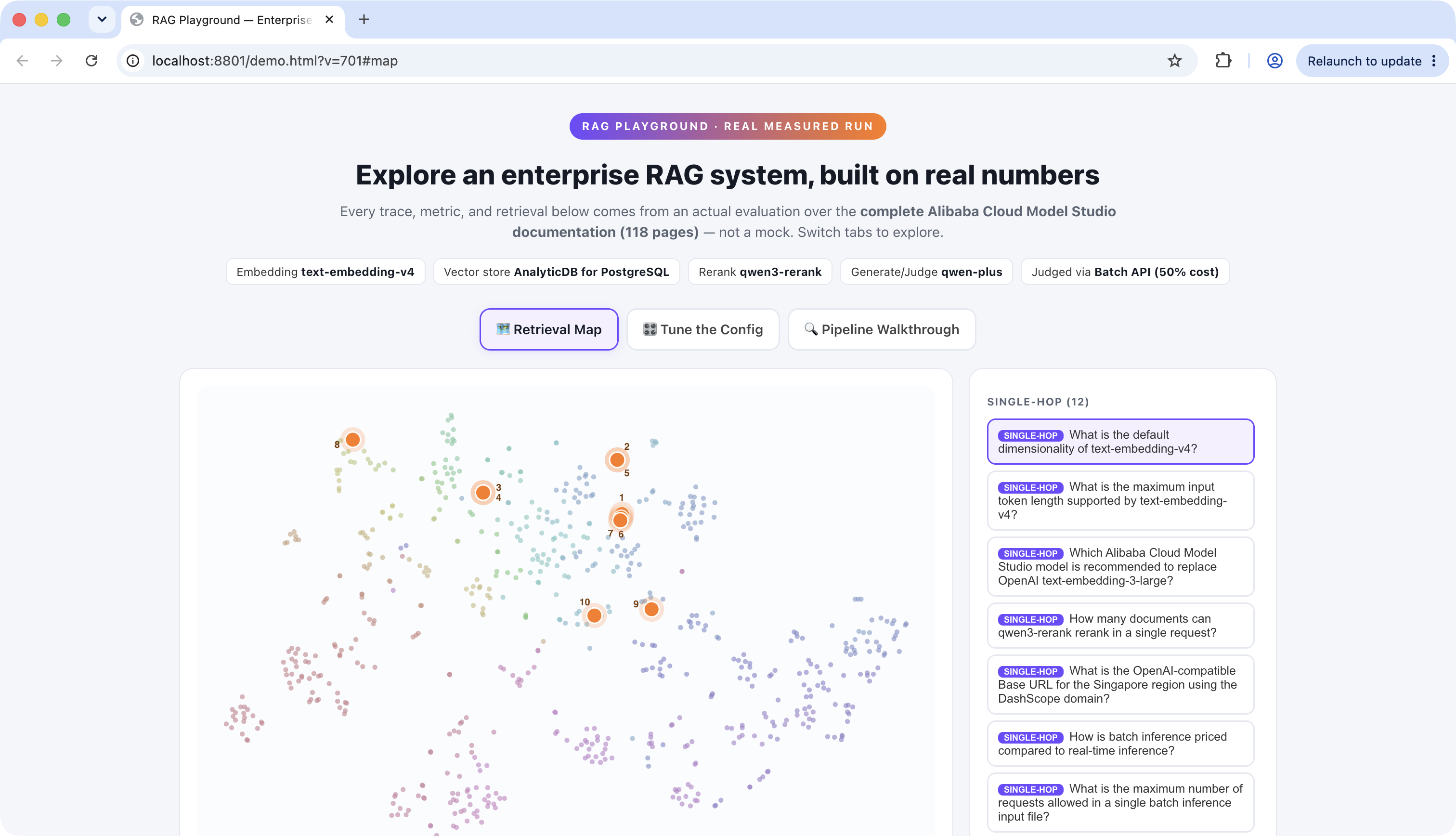
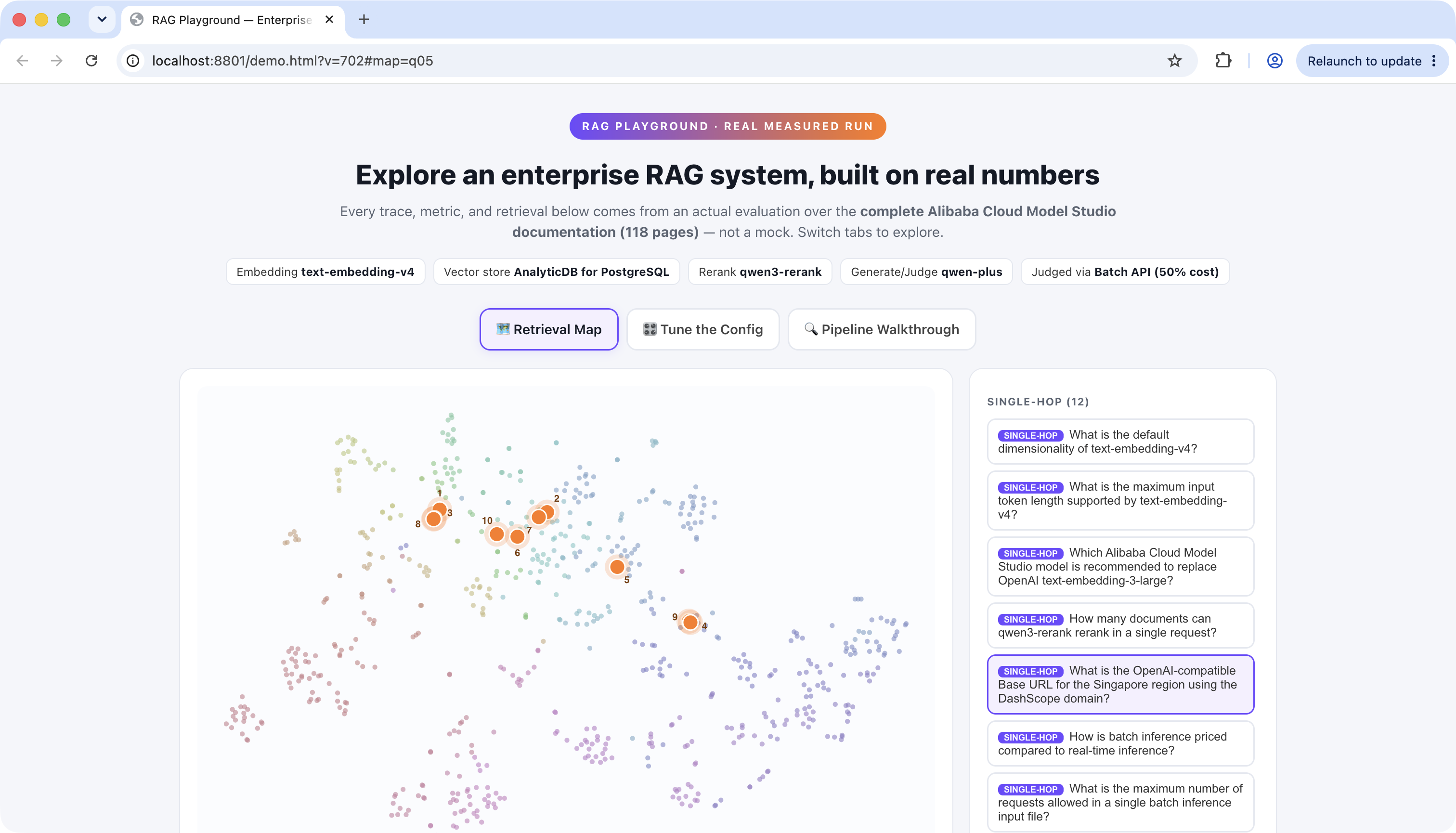
Retrieval Map. All 676 chunks of the corpus, projected into 2-D by t-SNE and colored by source document. Pick any of the 36 golden questions and watch vector search light up the exact chunks it retrieved (orange, ranked), with the golden-source document ringed in green. It is the most intuitive way to see what retrieval is doing and where it misses.
Tune the Config. Slide chunk size, top-k, and the reranker on/off and read the measured recall / accuracy / groundedness for that exact combination off the heatmap.
Pipeline Walkthrough. Step through any question from retrieval to reranking, generation, and judging. You can inspect the retrieved chunks, the highlighted golden sources, and the judge's verdict. Here are a correct answer and a refusal:
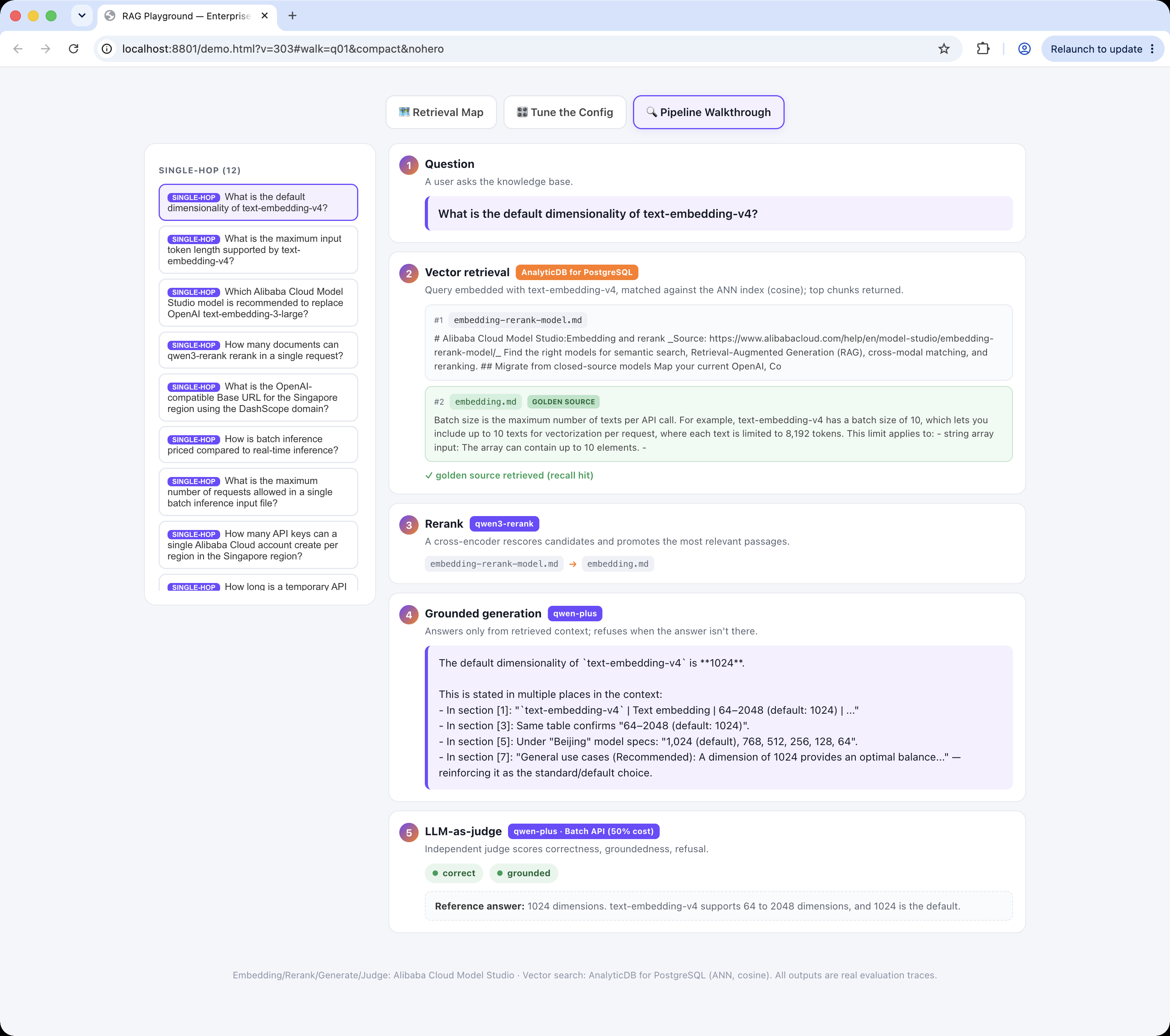

The answer: retrieval finds the golden document and qwen-plus answers 1024, confirmed correct + grounded. The refusal: an unanswerable question answered with "Not found in the knowledge base" instead of being invented.
qwen-plus), which raises a self-preference concern. To bound it, I re-judged the best combo's answers with an independent judge model (qwen-max): agreement was 30/30 on correctness and 6/6 on refusal (the 30 answerable and the 6 unanswerable questions respectively). That does not prove the judgments are human-correct, but it shows they are not an artifact of the model grading itself favorably.qwen-plus). Swap the model in config and re-run. That comparison is exactly what the harness is for.You do not need to guess your RAG settings, and you do not need to run your own GPU fleet or vector database to get a production-grade pipeline. With Model Studio for the models, AnalyticDB for PostgreSQL for vector search, and a disciplined evaluation loop that includes a golden set, deterministic recall, and LLM judging via the Batch API, you get a system whose accuracy you can state, not just hope for.
The reusable pieces, including the harness, the golden set, and the interactive playground, are yours to keep. Design "how do I know it's accurate" with the same care you put into "which model do I pick." Also Measure it!
References
Korean Version :Click
Alibaba Cloud
Hosung Kim | Sr.Technical Account Manager

6 posts | 1 followers
FollowAlibaba Cloud Data Intelligence - June 20, 2024
ApsaraDB - July 9, 2025
Data Geek - February 25, 2025
Alibaba Cloud Native Community - October 15, 2025
Alibaba Cloud Community - November 5, 2024
Alibaba Cloud Indonesia - April 14, 2025
6 posts | 1 followers
Follow AnalyticDB for PostgreSQL
An online MPP warehousing service based on the Greenplum Database open source program
Learn More Vector Retrieval Service for Milvus
A cloud-native vector search engine that is 100% compatible with open-source Milvus, extensively optimized in performance, stability, availability, and management capabilities.
Learn More AnalyticDB for MySQL
AnalyticDB for MySQL is a real-time data warehousing service that can process petabytes of data with high concurrency and low latency.
Learn More PolarDB for PostgreSQL
Alibaba Cloud PolarDB for PostgreSQL is an in-house relational database service 100% compatible with PostgreSQL and highly compatible with the Oracle syntax.
Learn MoreMore Posts by Hosung Kim

