Machine vision, or computer vision, is a popular research topic in artificial intelligence (AI) that has been around for many years. However, machine vision still remains as one of the biggest challenges in AI. In this article, we will explore the use of deep neural networks to address some of the fundamental challenges of computer vision. In particular, we will be looking at applications such as network compression, fine-grained image classification, captioning, texture synthesis, image search, and object tracking.
Even though deep neural networks feature incredible performance, their demands for computing power and storage pose a significant challenge to their deployment in actual application. Research shows that the parameters used in a neural network can be hugely redundant. Therefore, a lot of work is put into increasing accuracy while also decreasing the complexity of the network.
Low-rank approximation gets used to coming closer to the original weight matrix. For example, SVD can be used to obtain the optimal low-rank approximation of the matrix, or a Toeplitz matrix can be used in conjunction with a Krylov analysis to approximate the original matrix.
Once training is complete, some irrelevant neuron connections (can weight value balancing and sparse constraints in the loss algorithm), or filter all of them out, then execute several rounds of fine-tuning. In actual application, pruning the level of neuron connections will make the results sparse, difficult to cache, and difficult to access from memory. Sometimes, we need to design a cooperative operations database especially.
By comparison, filter-level pruning can get to run directly on the already present operation database, and the key to filter-level pruning is determining how to balance the importance of the filter. For example, we can use the sparsity of the results from convolution, the impact of the filter on the loss algorithm, or the impact of the convolution on the results of the next layer for balancing.
We can separate weight values into groups, and then use the median value in a group to replace the original weight, and run it through Huffman encoding. This can include scalar quantization or product quantization. However, if we only take the weights themselves into consideration, then the error deviation of the quantization process can get reduced. Subsequently, the error deviation of classification operations would get increased significantly. Therefore the optimization goal of Quantized CNN is to restructure to minimize the error deviation. Furthermore, we can use hash encoding and projected same hash bucket weights to share the same value.
Under the default circumstances, the data is composed of single precision floating points, taking up 32 bits. Researchers have discovered that using a half-precision floating point (16 bits) has nearly zero impact on performance. Google's TPU uses 8-bit integers to represent data. The final situation is that the range of values is either two or three values (0/1 or -1/0/1). Using only bits for operation can allow us to complete all kinds of computation quickly, however training a two or three value network is a vital issue.
The conventional method is to use two or three values for the feed-forward process and pass real numbers in the updating process. Furthermore, researchers believe that the expressive ability of two value operations is limited, so it uses an extra floating-point scaling binary convolution result to improve network representation.
Researchers have worked on creating a simplified network structure. For example,
Knowledge distillation training a small network to approach an extensive network. However, it is still unclear how correctly to approach a vast network.
There are two main types of commonly used hardware:
Compared to (common) image classification, fine-grained image classification requires more precision in determining the class of an image. For example, we might need to determine the exact species of the target bird, the make, and model of a car, or the model of an airplane. Normally, the differences between these kinds of classes are minimal. For example, the only outwardly visible difference between a Boeing 737-300 and a Boeing 737-400 is the number of windows. Therefore, fine-grained image classification is an even more challenging task than standard image classification.
The classic method of fine-grained image classification is to first define different locations on the image, for example, the head, foot, or wings of a bird. Then we have to extract features from these locations, and finally, combine these features and use them to complete classification. This type of method features very high accuracy, but it requires a massive dataset and manual tagging of location information. One major trend in fine-grained classification is training without additional supervision information, instead of using only image notes. This method gets represented by the bilinear CNN method.
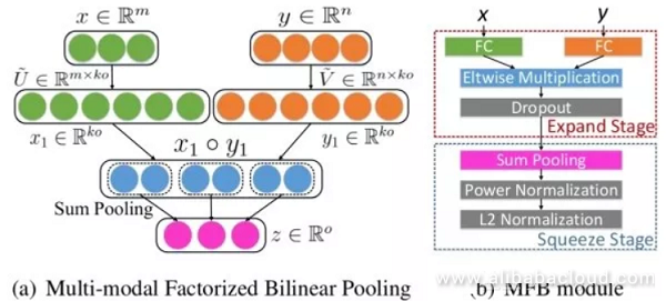
This computes the outer-product of convolution descriptors to find the mutual relationships between different dimensions. Because the dimensions of different descriptors correspond to different channels for convolution features, and different channels extract different semantic features, using bilinear operation allows us to capture the relationships between different semantic elements on the input image.

The result of bilinear confluence is exceptionally high-dimensional. This requires a significant amount of computing and storage resources, also significantly increased the number of parameters on the next fully-connected layer. Follow-up research has aimed to create a strategy for streamlining bilinear confluence, the results of which include the following:
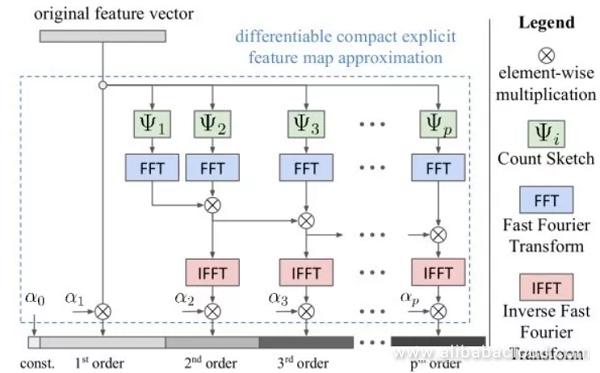
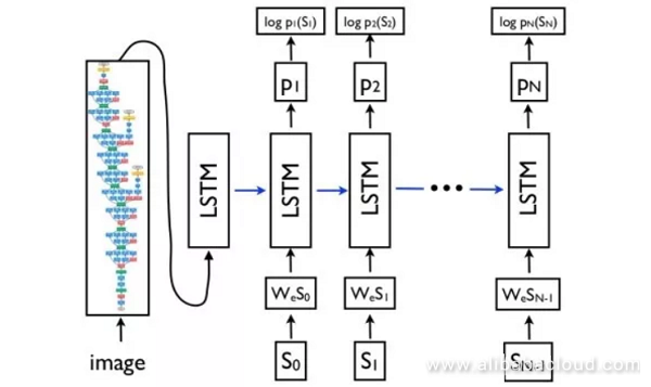
Image captioning is the process of generating a one or two sentence description of an image. This is a cross-disciplinary task that involves both vision and natural language processing.
The basic idea behind designing an image captioning network gets based on the concept behind machine translation in the field of natural language processing. After replacing the source language encoding network in a machine translator with an image CNN encoding network and extracting the features of the image, we can use the decoder network for the target language to create a text description.
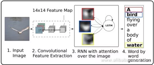
The Attention Mechanism is a standard technique used by machine translators to capture distant dependencies, and can also get used for image captioning. In the decoder network, at each moment, aside from predicting the next word, we also need to output a two-dimensional attention image and use it for weighted convergence of deep convolution features. An additional benefit to using an Attention Mechanism is that the network can get visualized so that we can easily see which part of the image the network was looking at when it produced each word.
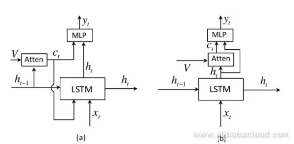
Previous Attention Mechanisms would produce a two-dimensional attention image for each predicted word (image(a)). However, for stop words like the, or, of, we do not need to use clues from the image. Instead, some words can get produced according to the context, completely independent of the image itself. This work expanded on LSTM and gave rise to the "visual sentry" mechanism which determines whether the current word should get predicted according to context or the image information (image(b)).
Furthermore, unlike the previous method which computed the attention image according to the state of the hidden layer at an earlier instance, this method performs calculations according to the current state of the hidden layer.
Given an image and a question related to that image, visual question answering aims to answer that question from a selection of candidate answers. In its essence, this is a classification task, and sometimes it uses recursive neural network decoding to produce the text answer. Visual question answering is also a cross-disciplinary task that involves both vision and natural language processing.
The concept is to use CNN to extract features from an image, RNN to extract text features from the text question, then combine the visual and textual features, and finally perform classification using the fully-connected later. The key to this task is figuring out how to connect these two types of features. Methods that directly combine these features transform them into a vector, or add or produce the visual and textual vector by adding or multiplying the elements.
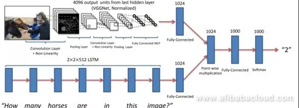
Attention Mechanisms like in image captioning systems, using an Attention Mechanism increases the performance of visual question answering. Attention Mechanisms include visual attention ("where am I looking") and textual attention ("which word am I looking at?") HieCoAtten can create visual and textual attention either at the same time or in turn. DAN projects the results of visual and textual attention in the same space; then it concurrently produces the next step in visual and textual attention accordingly.
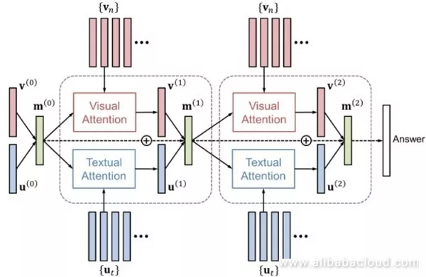
This method uses the outer product of visual feature vectors and textual feature vectors to capture the relationships between the features of these states on every dimension. To avoid explicitly computing the highly-dimensional result of bilinear confluence, we can apply the thought behind streamlined bilinear confluence found in fine-grained recognition to visual question answering. For example, MFB uses the concept behind low rate approximation as well as visual and textual attention mechanisms.
These methods provide many visualization methods to aid in understanding convolution and neural networks.
Since the filter on the first convolution layer slides on the input image, we can directly visualize the filter on the first layer. We can see that the first layer of weight focuses on the edge in a specific direction and a specified combination of colors. This is similar to visual biological mechanisms. However, since the high-level filter is not used directly on the input image, direct visualization can only be applied to the filter on the first layer.
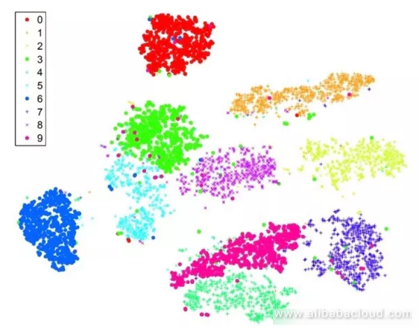
This method uses low-dimensional embedding on the fc7 and pool5 features of the image. For example, reducing them down to 2 dimensions allows them to be drawn on a 2-dimensional plane. Images with similar semantic information should yield similar results from t-SNE. The difference between this method and PCA is that t-SNE is a non-linear reduction method that preserves the distance between localities. We arrive at the following image which is the result of applying t-SNE to the original MNIST image. We can see that MNIST is a relatively simple dataset where differences between images of different classifications are obvious.
Draw different feature image responses for a specific input image. We can see that even though ImageNet does not have a category for human faces, the network will still learn to distinguish between this semantic information and capture future classifications.
To impelement this, select a specified neuron in the middle layer, then input multiple different images to the network to find the image region that causes the maximum response from the neuron. This allows us to observe which semantic feature the neuron corresponds to. The reason that we use "image regions" and not "the complete image" is that receptive field of a middle layer neuron is limited and cannot cover the entire image.
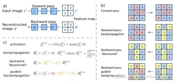
Input Saliency Map calculates the partial derivative produced by a specific neuron in reaction to a given input image. This represents the impact that different pixels in the picture have on the response of the neuron to that image and the changes to the reaction that are produced by changes to those pixels. Guided backdrop only back-propagates positive gradient values and only pays attention to positive influences on the neuron. This will create an even better visualization effect than standard back-propagation.
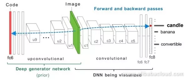
This method selects a specific neuron and then calculates the partial derivative produced by that neuron in reaction to the input image, then optimizes the image using gradient rise until convergence. Furthermore, we need some normalized items to bring the produced image closer to the natural model. Aside from optimizing the input image, we can also optimize the fc6 feature and create the required image.
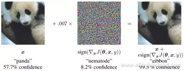
Selects an image and an incorrect classification for it. The system then computes the partial derivative of that classification to the image and then applies gradient rise optimization to the image. Experiments show that after using a small, nigh imperceptible change, we can cause the network to implement the incorrect class to the model with high confidence.
In practical application, adversarial examples are significantly helpful in the fields of finance and security. Researchers have found that this is because that the image space is very highly-dimensional. We can only cover a small part of that space even with a vast amount of training data. If the input picture varies even a little bit from that different space, then it will be difficult for the network to reach a reasonable decision.
Announcing July's Winners and Best Entries of the Alibaba Cloud Community Builder Program
Deep Dive into Computer Vision with Neural Networks – Part 2

2,593 posts | 793 followers
FollowAlibaba Clouder - November 4, 2019
Alibaba Clouder - August 10, 2018
Alibaba Clouder - October 29, 2019
Alibaba Clouder - November 5, 2019
Alibaba Clouder - May 6, 2020
Alibaba F(x) Team - June 20, 2022

2,593 posts | 793 followers
Follow Image Search
An intelligent image search service with product search and generic search features to help users resolve image search requests.
Learn More E-MapReduce Service
A Big Data service that uses Apache Hadoop and Spark to process and analyze data
Learn More MaxCompute
Conduct large-scale data warehousing with MaxCompute
Learn MoreMore Posts by Alibaba Clouder
5506072527090541 October 31, 2019 at 1:14 pm
Very nice article!!! Do you want to know about Challenges in computer vision please check this article https://blog.skyl.ai/what-is-computer-vision/ i would love take some suggestion