By Xixia
What is machine learning? First, let's look at two examples.
Imagine people who have never seen a cat, such as little babies. They do not even have the word "cat" in their vocabulary.
One day they see a furry animal like this:

They do not know what it is, and you tell them that it is a "cat". At this time, they may remember that it is a cat.
After some time, they see another animal like this:

You tell them that it is also a cat. They remember that it is also a cat.
Later on, they see another animal:

At this time, they tell you directly that they see a "cat".
The preceding method is the basic method that we use to understand the world, which is pattern recognition: We concluded that it is a cat based on extensive experiences.
In this process, we learned about the characteristics of cats by contacting samples, which are various cats. We learn through reading and observe how they mew, and what they look like with two ears, four legs, a tail, and whiskers, to draw the conclusion. Then, we know what a cat is.
The following is a piece of code written by one of my colleagues:
SELECT * FROM
  tianma.module_xx
WHERE
  pt = TO_CHAR(DATEADD(GETDATE(), - 1, 'dd'), 'yyyymmdd')
  AND name NOT LIKE '%test%'
  AND name NOT LIKE '%demo%'
  AND name NOT LIKE '%测试%'
  AND keywords NOT LIKE '%test%'
  AND keywords NOT LIKE '%测试%'
  AND keywords NOT LIKE '%demo%'
Obviously, our criterion is whether the module's name and keywords contain characters: test or demo. If it is true, we consider it as a test module. We tell the database our rules, and the database helps us filter out non-test modules.
The identification of a cat is essentially the same as the identification of a test module. Both imply looking for characteristics:
The characteristics can be further programmed as follows:
With these characteristics, both people and machines can recognize a cat or a test module.
To put it simply, machine learning uses characteristics and their weights to implement data classification. This simplified statement is for your ease of understanding. For more information, see AiLearning/1. Basic Machine Learning.md at master apachecn/AiLearning at GitHub.
The reason is that when a classification task involves large amounts of characteristics, it is difficult to use "if-else" to perform simple classification. Take our common product recommendation algorithm as an example. To identify whether a certain product should be recommended to someone, the algorithm may involve hundreds of characteristics.
Data preparation may account for more than 75% of the time consumed by the entire machine learning task. Therefore, it is the most important and most difficult part. The main steps are as follows:
1) Collect basic data.
2) Remove outliers.
3) Select possible characteristics: characteristic engineering.
4) Tag the data.
Fit your data with a function: y = f(x)
For example, use a linear function: y = ax + b
Use an evaluation function to find out whether you have found the proper 'a' and 'b' values.
An evaluation function describes the difference between the parameters that are obtained through training and the actual values. The difference is also called loss value. The following figure shows an example:
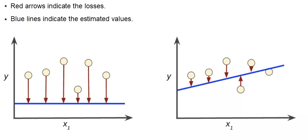
The blue line on the right is closer to the actual data points.
The most common loss evaluation function is the mean squared error. This function measures the average squared difference between the estimated values and the actual value to judge the quality of estimated values.
As shown in the preceding figure, the coordinates of the small yellow circles in the sample are as follows:
[
[x1, y1],
[x2, y2],
[x3, y3],
[x4, y4],
[x5, y5],
[x6, y6]
]
The estimated coordinates on the blue line are as follows:
[
[x1, y'1],
[x2, y'2],
[x3, y'3],
[x4, y'4],
[x5, y'5],
[x6, y'6]
]
Therefore, the loss value is:
const cost = ((y'1-y1)^2 + (y'2-y2)^2 + (y'3-y3)^2 + (y'4-y4)^2 + (y'5-y5)^2 + (y'6-y6)^2 )/6Taking the preceding linear function as an example. Training an algorithm is actually looking for the proper values of 'a' and 'b'. If we perform a random search in the vast ocean of numbers, we will never find the proper values of 'a' and 'b'. In this case, we need to use a gradient descent algorithm to find the proper values of 'a' and 'b'.
To clarify the goal, replace the preceding formula for calculating the loss value with y = ax + b
// Function 2
const cost = (((a*x1+b)-y1)^2 + ((a*x2+b)-y2)^2 + ((a*x3+b)-y3)^2 + ((a*x4+b)-y4)^2 + ((a*x5+b)-y5)^2 + ((a*x6+b)-y6)^2 )/ 6
Our goal is to find the 'a' and 'b' values that minimize the cost. With this goal, we may go straight to find a solution.
Do you still remember the quadratic functions you learned in middle school, which are quadratic equations: y = ax^2 + bx + c?
Although the preceding cost function seems long, it is also a quadratic function. Its graph is probably as follows:
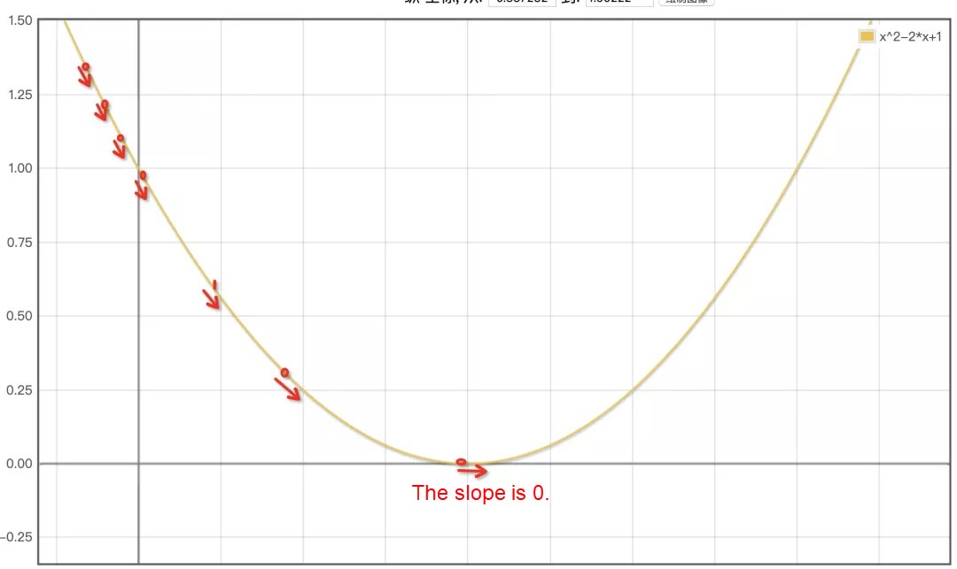
As long as we can find the 'a' and 'b' values for the lowest point, we can achieve our goal.
Let's assume we randomly initialize the value of 'a' as 1, then the point is on the upper-left part of the parabola, and it is still far away from the lowest point with the minimum cost.
As shown in the preceding figure, we only need to increase the value of 'a' to approach the lowest point. However, machines are unable to understand the graph. In this case, we look to the most complicated mathematical knowledge in this article: derivative. At this point, the slope of the tangent line is the derivative of this parabola, such as the lowest point (the slope is 0) in the preceding graph.
We can calculate the slope of the tangent line (the oblique red line) here through this derivative. If the slope of this oblique line is negative, it means that the value of a is too small and needs to be increased to get closer to the bottom. On the contrary, if the slope is positive, it means that the value of 'a' has passed the lowest point and needs to be reduced to get closer to the bottom.
Let's look at the following code. To understand the code, first review the mathematical knowledge: partial derivative and how to find the derivative of composite functions.
// Function 3
// Partial derivative of a
const costDaoA = (((a*x1+b)-y1)*2*x1 + ((a*x2+b)-y2)*2*x1 + ((a*x3+b)-y3)*2*x1 + ((a*x4+b)-y4)*2*x1 + ((a*x5+b)-y5)*2*x1 + ((a*x6+b)-y6)*2*x1 )/ 6

// Partial derivative of b
const costDaoB = (((a*x1+b)-y1)*2 + ((a*x2+b)-y2)*2 + ((a*x3+b)-y3)*2 + ((a*x4+b)-y4)*2 + ((a*x5+b)-y5)*2 + ((a*x6+b)-y6)*2 )/ 6
If we bring the 'a' and 'b' values into the costDaoA function, we get a slope, which determines how to adjust the parameter 'a' to get closer to the bottom.
Similarly, costDaoB determines how to adjust the parameter 'b' to get closer to the bottom.
If you run for 500 cycles in this way, you can get very close to the bottom and obtain the proper 'a' and 'b' values.
Obtain a model like y = ax + b, which we can use to make estimations.
It is known to all that crickets chirp more frequently in hot weather than in cool weather. We have recorded the temperatures and the cricket chirps per minute in a table and graphed the table in Excel as follows (The case is from the official tutorial of Google TF):
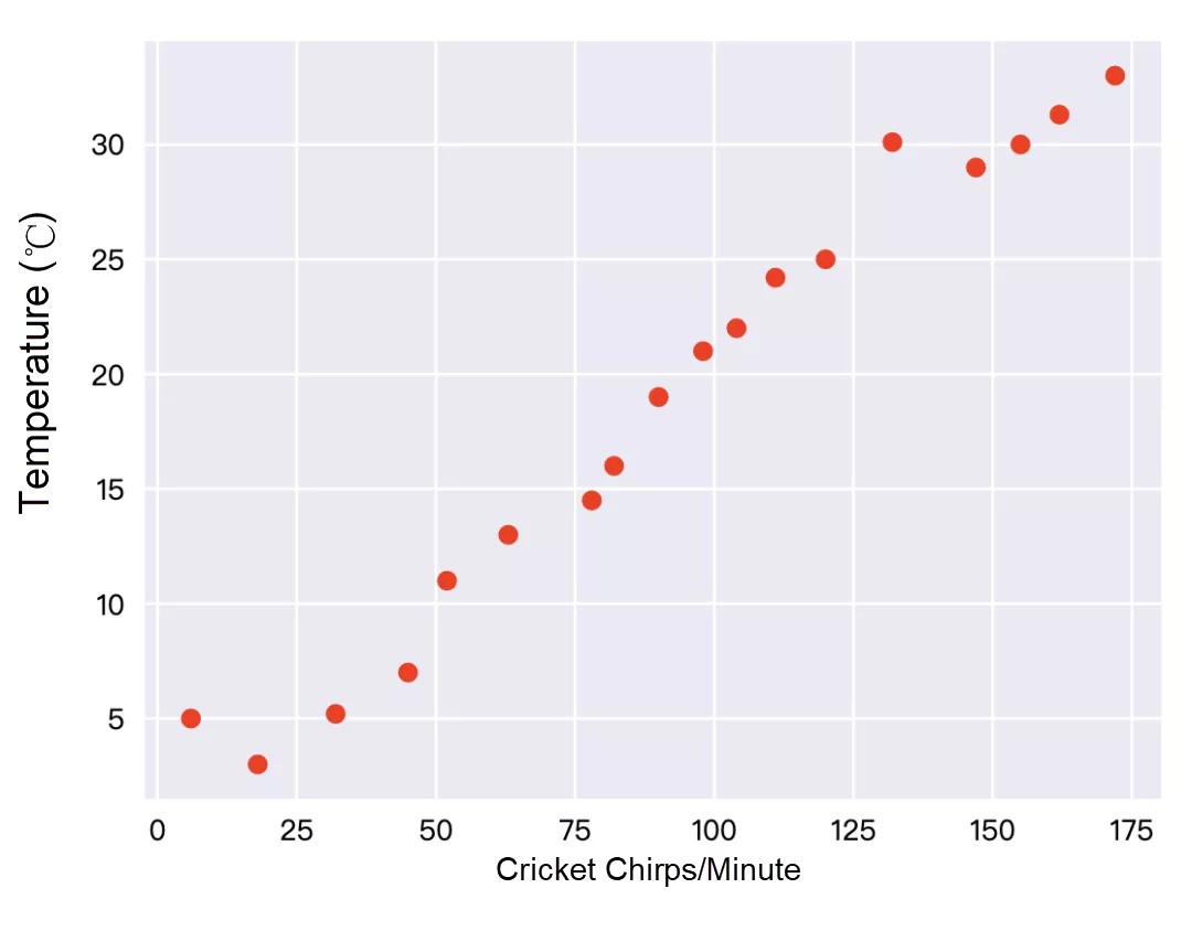
It is clear that these red dots are almost on a straight line:
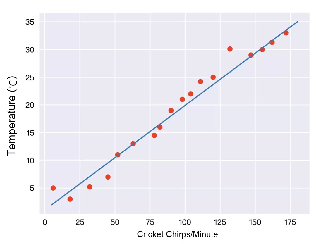
Therefore, we regard the data distribution as linear, and the process of drawing this straight line is called linear regression. With this straight line, we accurately estimate the cricket chirps per minute under any circumstances.
Address: test gradient descent
https://jshare.com.cn/feeqi/CtGy0a/share?spm=ata.13261165.0.0.6d8c3ebfIOhvAq
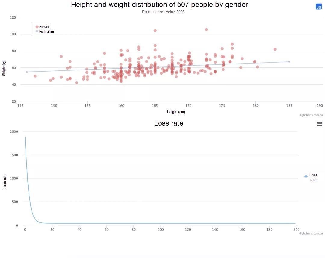
We use highcharts for data visualization and directly use the default data points of highcharts to save 75% of the time consumed.
When the training is completed, a blue line is overlaid on the graph, and the loss rate curve of 'a' and 'b' values for each training cycle are added.
/**

* Cost function and calculation of the mean squared error

*/

function cost(a, b) {

    let sum = data.reduce((pre, current) = >{

        return pre + ((a + current[0] * b) - current[1]) * ((a + current[0] * b) - current[1]);

    },
    0);

    return sum / 2 / data.length;

}

/**

* Calculate the gradient

* @param a

* @param b

*/

function gradientA(a, b) {

    let sum = data.reduce((pre, current) = >{

        return pre + ((a + current[0] * b) - current[1]) * (a + current[0] * b);

    },
    0);

    return sum / data.length;

}

function gradientB(a, b) {

    let sum = data.reduce((pre, current) = >{

        return pre + ((a + current[0] * b) - current[1]);

    },
    0);

    return sum / data.length;

}

// Number of training cycles
let batch = 200;

// This is the speed at which the result value gets closer to the bottom in each cycle. It is also the learning speed. If it is too high, the result value will bounce around the lowest point. If the speed is too low, the learning efficiency will become lower.
let alpha = 0.001;

let args = [0, 0]; // Initialized a and b values
function step() {

    let costNumber = (cost(args[0], args[1]));

    console.log('cost', costNumber);

    chartLoss.series[0].addPoint(costNumber, true, false, false);

    args[0] -= alpha * gradientA(args[0], args[1]);

    args[1] -= alpha * gradientB(args[0], args[1]);

    if ((—batch > 0)) {

        window.requestAnimationFrame(() = >{
            step()
        });

    } else {

        drawLine(args[0], args[1]);

    }

}

step();When there are more characteristics, we need to perform more calculations and invest more time in training to obtain a training model.
After you read the preceding simple descriptions, machine learning is now definitely no longer mysterious to you. Refer to the introductory articles that are more professional.
If you're interested to start your AI/ML journey on Alibaba Cloud, please visit the Machine Learning Platform for AI (PAI) page to learn more.
References
1) GitHub - apachecn/AiLearning: AiLearning: Machine Learning - MachineLearning - ML, Deep Learning - DeepLearning - DL, Natural Language Processing - NLP
2) https://developers.google.com/machine-learning/crash-course/descending-into-ml/video-lecture?hl=zh-cn
3) Learn Machine Learning from Zero: A Step-by-step Guide to the Implementation of Gradient Descent with Python
The views expressed herein are for reference only and don't necessarily represent the official views of Alibaba Cloud.

2,593 posts | 793 followers
FollowAlibaba F(x) Team - December 11, 2020
Alibaba Container Service - July 29, 2019
GarvinLi - November 7, 2018
Alibaba F(x) Team - December 8, 2020
Alibaba F(x) Team - September 1, 2021
Alibaba F(x) Team - June 22, 2021

2,593 posts | 793 followers
Follow Offline Visual Intelligence Software Packages
Offline SDKs for visual production, such as image segmentation, video segmentation, and character recognition, based on deep learning technologies developed by Alibaba Cloud.
Learn More Network Intelligence Service
Self-service network O&M service that features network status visualization and intelligent diagnostics capabilities
Learn More Database for FinTech Solution
Leverage cloud-native database solutions dedicated for FinTech.
Learn More Oracle Database Migration Solution
Migrate your legacy Oracle databases to Alibaba Cloud to save on long-term costs and take advantage of improved scalability, reliability, robust security, high performance, and cloud-native features.
Learn MoreMore Posts by Alibaba Clouder