Optimization Solver:Optimization Solver User Guide

Command line call example

On Linux and macOS, assume that you have installed MindOpt to the directory specified by the `$MINDOPT_HOME` environment variable as described in the installation document:

mindopt $MINDOPT_HOME/examples/data/afiro.mps

On Windows:

mindopt %MINDOPT_HOME%\examples\data\afiro.mps

C/C++/C#/Java/Python/MATLAB call example

V1.x

env = mindoptpy.Env()
env.start()
model = mindoptpy.read(filename, env)
model.optimize()
print(f"Optimal objective value is: {model.objval}")
for v in x:
    print(f"{v.VarName} = {v.X}")

MDOEnv env = new MDOEnv();
MDOModel model = new MDOModel(env, filename);
model.optimize();
System.out.println("Optimal objective value is: " + model.get(MDO.DoubleAttr.ObjVal));
MDOVar[] x = model.getVars();
for (int i = 0; i < x.length; ++i) {
    System.out.println(x[i].get(MDO.StringAttr.VarName) + " = " + x[i].get(MDO.DoubleAttr.X));
}

MDOEnv env = MDOEnv();
MDOModel model = MDOModel(env, filename);
model.optimize();
std::cout << "Optimal objective value is: " << model.get(MDO_DoubleAttr_ObjVal) << std::endl;
std::vector<MDOVar> vars = model.getVars();
for (auto v : vars) {
    std::cout << v.get(MDO_StringAttr_VarName) << " = " << v.get(MDO_DoubleAttr_X) << std::endl;
}

MDOenv* env;
MDOemptyenv(&env);
MDOstartenv(env);
MDOmodel* model;
double obj;

MDOreadmodel(env, argv[1], filename);
MDOoptimize(model);
MDOgetdblattr(model, MDO_DBL_ATTR_OBJ_VAL, &obj);
printf("Optimal objective value is: %f\n", obj);

/* Free the environment. */
MDOfreemodel(model);
MDOfreeenv(env);

MDOEnv env = new MDOEnv();
MDOModel model =new MDOModel(env, filename);
model.optimize();
Console.WriteLine($"Optimal objective value is: {model.Get(MDO.DoubleAttr.ObjVal)}");
MDOVar[] vars = model.GetVars();
for (int i = 0; i < vars.Length; i++)
{
    Console.WriteLine($"{vars[i].Get(MDO.StringAttr.VarName)} = {vars[i].Get(MDO.DoubleAttr.X)}");
}

model = mindopt_read(file);
result = mindopt(model);

for v=1:length(result.X)
    fprintf('%s %d\n', model.varnames{v}, result.X(v));
end
fprintf('Optimal objective value is: %e\n', result.ObjVal);

objval = result.ObjVal;

For complete code examples, see More.

V0.x

# Method 1: A new model creation method was introduced in version 0.19.0. This method provides faster cloud authentication and consumes less concurrency.
env = mindoptpy.MdoEnv()
model = mindoptpy.MdoModel(env)
model.read_prob(filename)
model.solve_prob()
model.display_results()

# Method 2: The old model creation method is still supported.
# model = mindoptpy.MdoModel()
# model.read_prob(filename)
# model.solve_prob()
# model.display_results()

//<dependency>
//    <groupId>com.alibaba.damo</groupId>
//    <artifactId>mindoptj</artifactId>
//    <version>[0.20.0,)</version>
//</dependency>
// Load the dynamic-link library, as follows:
Mdo.load("c:\\mindopt\\0.20.0\\win64_x86\\lib\\mindopt_0_20_0.dll");

// Method 1: A new model creation method was introduced in version 0.19.0. This method provides faster cloud authentication and consumes less concurrency.
// Set up the environment during program initialization, for example, in the setup phase of MapReduce.
MdoEnv env = new MdoEnv();
// Create a model.
MdoModel model = env.createModel();
model.readProb(filename)
model.solveProb();
model.displayResult();
model.free();
// The Java SDK requires you to manually release the env at the end of the program, for example, in the cleanup phase of MapReduce.
env.free();

// Method 2: The old model creation method is still supported but is marked as deprecated and will be removed in a future version.
/*
MdoModel model = new MdoModel();
model.readProb(filename)
model.solveProb();
model.displayResult();
*/

// Method 1: A new model creation method was introduced in version 0.19.0. This method provides faster cloud authentication and consumes less concurrency.
using mindopt::MdoEnv;
MdoEnv env;
MdoModel model(env);
model.readProb(filename);
model.solveProb();
model.displayResults();

// Method 2: The old model creation method is still supported.
/*
MdoModel model;
model.readProb(filename);
model.solveProb();
model.displayResults();
*/

// Method 1: A new model creation method was introduced in version 0.19.0. This method provides faster cloud authentication and consumes less concurrency.
MdoEnvPtr env;
MdoMdlPtr model;
Mdo_createEnv(&env);
Mdo_createMdlWithEnv(&model, env);
Mdo_readProb(model, filename);
Mdo_solveProb(model);
Mdo_displayResults(model);
Mdo_freeMdl(&model);
// The C SDK requires you to manually release the env.
Mdo_freeEnv(&env);

// Method 2: The old model creation method is still supported.
/*
MdoMdlPtr model;
Mdo_createMdl(&model);
Mdo_readProb(model, filename);
Mdo_solveProb(model);
Mdo_displayResults(model);
Mdo_freeMdl(&model);
*/

For complete code examples, see the V0.x documentation.

Method 1: File input

• The solver supports the MPS format and the LP format, such as .mps and .lp files, and their compressed versions, such as .mps.gz and .mps.bz2.

• The solver supports the .dat-s format, which is used in SDP problem examples.

• The solver supports the .qps format, which is used for QP problem data.

• The `mindoptampl` module supports .nl file input. For example, you can run the mindoptampl filename.nl command.

For more information, see More.

Method 2: Modeling API input

V1.x

Multiple related APIs are available that support row-wise data input.

• The following is a brief Python example:

  • Use mindoptpy.Model.modelsense = MDO.MINIMIZE to set the objective function to minimization.

  • Use mindoptpy.Model.addVar() to add optimization variables and define their lower bounds, upper bounds, objective coefficients, names, and types.

  • Use mindoptpy.Model.addConstrs() to add constraints.

For more information, see More. For a list of attributes, see More. The API chapters also contain complete examples for each language.

V0.x

Multiple related APIs are available, and the same data can be input in various ways.

• The following is a brief Python example for row-wise input:

  • Use mindoptpy.MdoModel.set_int_attr() to set the objective function to minimization.

  • Use mindoptpy.MdoModel.add_var() to add four optimization variables and define their lower bounds, upper bounds, names, and types.

  • Use mindoptpy.MdoModel.add_cons() to add constraints.

• The following is a brief Python example for column-wise input:

  • Use mindoptpy.MdoModel.set_int_attr() to set the objective function to minimization.

  • First, call mindoptpy.MdoModel.add_cons() to create constraints with specified left-hand and right-hand side values, but with no non-zero elements.

  • Create a temporary column object mindoptpy.MdoCol() to store the constraints and the values of non-zero elements sequentially.

  • Finally, call mindoptpy.MdoModel.add_var() to create new variables with their corresponding objective function coefficients, non-zero elements in the column vector, lower and upper bounds, variable names, and variable types.

For more information, see the V0.x documentation. For a list of model attributes, see the V0.x documentation.

Method 3: Modeling languages MindOpt APL, AMPL, Pyomo, PuLP, and JuMP

MindOpt supports several common modeling tools, including the following:

1. MindOpt APL

Support for MindOpt APL, a modeling language developed by the MindOpt team, was introduced in 2022.

• You can use the modeling language and solver for free in your browser on the MindOpt online modeling and solving platform. The platform also includes case studies to help you get started quickly. No software installation is required. You can open your browser to use it.

• For more syntax documentation, see More.

2. AMPL

Before using AMPL to call MindOpt, you must install MindOpt and AMPL. The `mindoptampl` application is located in the \bin\mindoptampl directory of the installation package. `mindoptampl` provides configurable parameters. You can use the AMPL option command to set the mindoptampl_options parameter. For example:

ampl: option mindoptampl_options 'numthreads=4 maxtime=1e+4';

For more information and examples, see More.

3. CVXPY

Before using CVXPY to call MindOpt, you must install MindOpt and CVXPY. To call the MindOpt solver's CVXPY API, you must first import the mindopt_conif.py and mindopt_qpif.py interface files. Import these files in your Python code as follows:

from mindopt_conif import *
from mindopt_qpif import *

For more information and examples, see More.

4. Pyomo

Before using Pyomo to call MindOpt, you must install MindOpt and Pyomo. To call the MindOpt solver's Pyomo API, you must use the mindopt_pyomo.py interface file. The MindOpt Pyomo interface inherits from Pyomo's DirectSolver class. The implementation code is in the \lib\pyomo\mindopt_pyomo.py file of the installation package. Import this file in your Python code as follows:

from mindopt_pyomo import MindoptDirect

For more information and examples, see More.

5. PuLP

Before using PuLP to call MindOpt, you must install MindOpt and PuLP. To call the MindOpt solver's PuLP API, you must use the mindopt_pulp.py interface file. The MindOpt PuLP interface inherits from PuLP's LpSolver class. The implementation code is in the \lib\pulp\mindopt_pulp.py file of the installation package. Import this file in your Python code as follows:

from mindopt_pulp import MINDOPT

For more information and examples, see More.

6. JuMP

JuMP is an open source modeling tool based on the Julia programming language. Before using JuMP to call MindOpt, you must install MindOpt, Julia, JuMP, and AmplNLWriter. Call the JuMP API to create a modeling object and specify `mindoptampl` as the solver.

model = Model(() -> AmplNLWriter.Optimizer(mindoptampl))

For more information, see More.

Reference for computing device configuration: Characteristics of different algorithms for LP solving

When you configure machine resources, the amount of resources consumed varies based on the problem structure and the selected algorithm. You should test and select the configuration as needed.

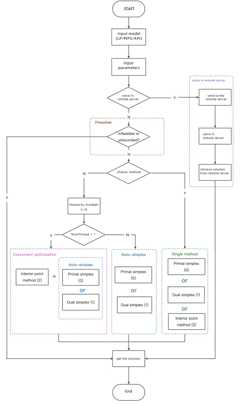
For LP solving, we currently provide the Simplex, Interior-Point Method (IPM), and Concurrent optimization algorithms. The execution flow is shown in the "Execution flow" image below. The Concurrent algorithm is selected by default. You can set the "Method" parameter to select a different algorithm.

The differences between these three algorithms are as follows:

Command line execution

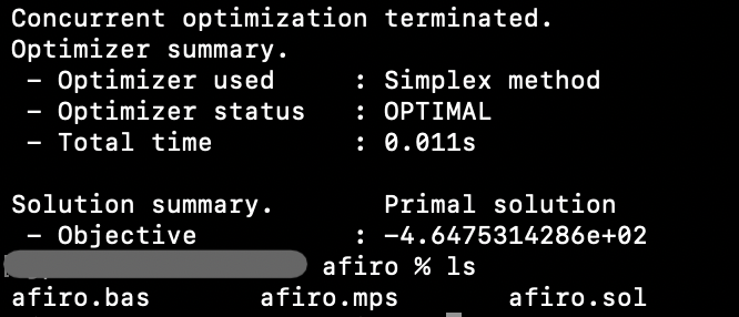
When you run the solver from the command line, it prints the output of the solving process and a summary of the results. It also generates .bas and .sol result files with the same name in the same directory as the problem file.

The following figure shows that after you run the mindopt afiro.mps command, the afiro.bas and afiro.sol files are generated in the folder. The .bas file saves the basis, and the .sol file saves the optimal objective value and the solution for the variable values.

API solving and result retrieval

V1.x

After you input the problem to be solved, call the optimize() API to solve it. For example, the Python command is model.optimize().

After solving, you can call APIs to retrieve the results. The following examples use Python:

• Call model.status to retrieve the solution status. Possible statuses include UNKNOWN, OPTIMAL, INFEASIBLE, UNBOUNDED, INF_OR_UBD, and SUB_OPTIMAL. For example, MDO.OPTIMAL in Python.

• Use model.objval to retrieve the objective value.

  • You can also call model.getAttr(MDO.Attr.PrimalObjVal) to retrieve other model attribute values. Similarly:

    • SolutionTime: Total running time in seconds

    • DualObjVal: Dual objective value

    • ColBasis: Basis of the primal solution

• Call var.X to retrieve the solution for a variable.

• For a list of more solution attributes, see More.

For complete code examples, see the `example` folder in the installation package, the documentation at More, or the examples chapter in each language's API documentation, such as the Python examples.

V0.x

After you input the problem to be solved, call the solveProb API to solve it. For example, the Python command is model.solve_prob().

After solving, you can call APIs to retrieve the results. The following examples use Python:

• Call model.display_results() to print the results.

• Call model.get_status() to retrieve the solution status.

• Call model.get_real_attr("PrimalObjVal") to retrieve the primal objective value. Similarly:

  • "DualObjVal": Dual objective value

  • "PrimalSoln": Primal solution

  • "ColBasis": Basis of the primal solution

  • For a list of more solution attributes, see the V0.x documentation

For complete code examples, see the `example` folder in the installation package or the documentation.

Infeasibility analysis for constraints

During the modeling and solving process, you may encounter infeasible problems caused by conflicting constraints. Analyzing the infeasible problem and identifying the key constraints that cause the conflict can significantly help with modeling. A minimal subset of constraints that causes the problem to be infeasible is called an irreduciable infeasible system (IIS).

MindOpt provides an API to compute an IIS. If a problem is "INFEASIBLE", you can use the compute IIS API to analyze the infeasible problem. For example, you can modify or remove the constraints in the IIS to make the optimization problem feasible.

The following is an example of how to call the IIS Python interface:

V1.x

if model.status == MDO.INFEASIBLE or model.status == MDO.INF_OR_UBD:
    idx_rows, idx_cols = model.compute_iis()

For complete instructions on computing an IIS, see More.

V0.x

status_code, status_msg = model.get_status()
if status_msg == "INFEASIBLE":
    idx_rows, idx_cols = model.compute_iis()

For complete instructions on computing an IIS, see the V0.x documentation.

MindOpt execution flow:

Different optimization problems have different solving methods, but the overall flow is similar. The following is an example of the call flow for an LP problem. During the process, you can set certain parameters.