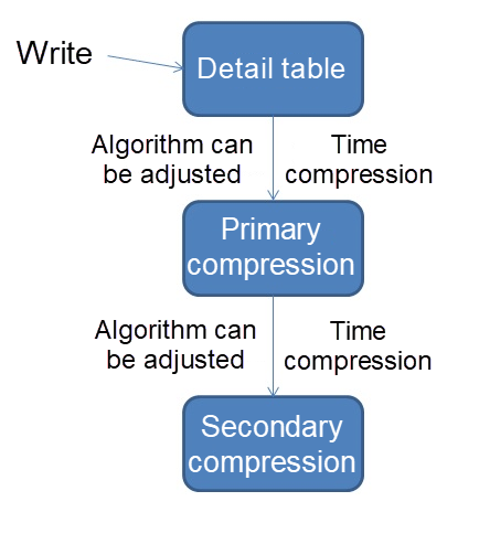
PostgreSQL Time-Series Data Case: Automatic Compression over Time

Background

One of the most important features of the time-series database is compression over time. For example, the data from the last day is compressed into a point of 5 minutes, and the data from the last week is compressed into a point of 30 minutes.

The PostgreSQL compression algorithm can be customized. For example, simple mean compression, maximum compression, and minimum compression; or compression based on the revolving door compression algorithm.

Implementation of the Revolving Door Data Compression Algorithm in PostgreSQL - Application of Streaming Compression in the IoT, Monitoring, and Sensor Scenarios

This article introduces a simple compression scenario, which is similar to an RRD database compressed into average, maximum, minimum, sum, number of records, and other dimensions according to the time dimension.

It also introduces advanced SQL usages such as window query, year-on-year comparison and period-over-period comparison UDF (including KNN calculation), and write uniformly by time.

Design

Detail Table

create table tbl (  
  id serial8 primary key,  -- primary key  
  sid int,                 -- sensor ID  
  hid int,                 -- indicator D  
  val float8,              -- collected value  
  ts timestamp             -- acquisition time 
);   
  
create index idx_tbl on tbl(ts);

Compression Table

1. 5-minute compression table

create table tbl_5min (  
  id serial8 primary key,  -- primary key 
  sid int,                 -- sensor ID  
  hid int,                 -- indicator ID  
  val float8,              -- inheritance, average, easy to do ring analysis  
  ts timestamp,            -- inheritance, start time, easy to do ring analysis
  val_min float8,              -- minimum  
  val_max float8,              -- maximum  
  val_sum float8,              -- and 
  val_count float8,            -- number of acquisitions 
  ts_start timestamp,      -- interval start time  
  ts_end timestamp         -- interval end time 
);   
  
alter table tbl_5min inherit tbl;

2. 30-minute compression table

create table tbl_30min (  
  id serial8 primary key,  -- primary key 
  sid int,                 -- sensor ID  
  hid int,                 -- indicator ID  
  val float8,              -- inheritance, average, easy to do ring analysis  
  ts timestamp,            -- inheritance, start time, easy to do ring analysis
  val_min float8,              -- minimum  
  val_max float8,              -- maximum  
  val_sum float8,              -- and 
  val_count float8,            -- number of acquisitions 
  ts_start timestamp,      -- interval start time  
  ts_end timestamp         -- interval end time 

);   
  
alter table tbl_30min inherit tbl;

3. 5-minute compression statement

with tmp1 as (  
  delete from only tbl where ts <= now()-interval '1 day' returning *  
)  
insert into tbl_5min  
  (sid, hid, val, ts, val_min, val_max, val_sum, val_count, ts_start, ts_end)   
select sid, hid, avg(val) as val, min(ts) as ts, min(val) as val_min, max(val) as val_max, sum(val) as val_sum, count(*) as val_count, min(ts) as ts_start, max(ts) as ts_end from   
tmp1  
group by sid, hid, substring(to_char(ts, 'yyyymmddhh24mi'), 1, 10) || lpad(((substring(to_char(ts, 'yyyymmddhh24mi'), 11, 2)::int / 5) * 5)::text, 2, '0');

4. 30-minute compression statement

with tmp1 as (  
  delete from only tbl_5min where ts_start <= now()-interval '1 day' returning *  
)  
insert into tbl_30min  
  (sid, hid, val_min, val_max, val_sum, val_count, ts_start, ts_end)  
select sid, hid, min(val_min) as val_min, max(val_max) as val_max, sum(val_sum) as val_sum, sum(val_count) as val_count, min(ts_start) as ts_start, max(ts_end) as ts_end from   
tmp1     
group by sid, hid, substring(to_char(ts_start, 'yyyymmddhh24mi'), 1, 10) || lpad(((substring(to_char(ts_start, 'yyyymmddhh24mi'), 11, 2)::int / 30) * 30)::text, 2, '0');

DEMO

1. 100 million pieces of detailed test data are written and distributed over 10 days.

insert into tbl (sid, hid, val, ts) select random()*1000, random()*5, random()*100,   – 1000 sensors and 5 indicators per sensor.  
  now()-interval '10 day' + (id * ((10*24*60*60/100000000.0)||' sec')::interval)   – push back for 10 days as the starting point + (id * time taken for each record)  
from generate_series(1,100000000) t(id);

2. 5-minute compression scheduling. For data from the last day, the following SQL is scheduled every 1 hour.

with tmp1 as (  
  delete from only tbl where ts <= now()-interval '1 day' returning *  
)  
insert into tbl_5min  
  (sid, hid, val, ts, val_min, val_max, val_sum, val_count, ts_start, ts_end)   
select sid, hid, avg(val) as val, min(ts) as ts, min(val) as val_min, max(val) as val_max, sum(val) as val_sum, count(*) as val_count, min(ts) as ts_start, max(ts) as ts_end from   
tmp1  
group by sid, hid, substring(to_char(ts, 'yyyymmddhh24mi'), 1, 10) || lpad(((substring(to_char(ts, 'yyyymmddhh24mi'), 11, 2)::int / 5) * 5)::text, 2, '0');

3. 30-minute compression scheduling. For data from the last week, the following SQL is scheduled every 1 hour.

with tmp1 as (  
  delete from only tbl_5min where ts_start <= now()-interval '1 day' returning *  
)  
insert into tbl_30min  
  (sid, hid, val_min, val_max, val_sum, val_count, ts_start, ts_end)  
select sid, hid, min(val_min) as val_min, max(val_max) as val_max, sum(val_sum) as val_sum, sum(val_count) as val_count, min(ts_start) as ts_start, max(ts_end) as ts_end from   
tmp1     
group by sid, hid, substring(to_char(ts_start, 'yyyymmddhh24mi'), 1, 10) || lpad(((substring(to_char(ts_start, 'yyyymmddhh24mi'), 11, 2)::int / 30) * 30)::text, 2, '0');

Summary

1. Group time by the interval and use integer division + multiplication.

Example:

5 minutes:

substring(to_char(ts, 'yyyymmddhh24mi'), 1, 10) || lpad(((substring(to_char(ts, 'yyyymmddhh24mi'), 11, 2)::int / 5) * 5)::text, 2, '0');

30 minutes:

substring(to_char(ts_start, 'yyyymmddhh24mi'), 1, 10) || lpad(((substring(to_char(ts_start, 'yyyymmddhh24mi'), 11, 2)::int / 30) * 30)::text, 2, '0')

2. Generate evenly distributed time-series data. The write time can be evenly distributed to the corresponding interval by using the interval and generate_series of PG.

insert into tbl (sid, hid, val, ts) select random()*1000, random()*5, random()*100,   – 1000 sensors and 5 indicators per sensor.  
  now()-interval '10 day' + (id * ((10*24*60*60/100000000.0)||' sec')::interval)   – push back for 10 days as the starting point + (id * time taken for each record)  
from generate_series(1,100000000) t(id);

3. One of the most important features of the time-series database is compression over time. For example, the data from the last day is compressed into a point of 5 minutes, and the data from the last week is compressed into a point of 30 minutes.

The PostgreSQL compression algorithm can be customized. For example, simple mean compression, maximum compression and minimum compression, or compression based on the revolving door compression algorithm.

Add scheduling:

PostgreSQL Scheduled Task Method 2

PostgreSQL Oracle Compatibility- DBMS_JOBS - Daily Maintenance - Timing Tasks (pgagent)

4. After compression, it contains the values of interval, maximum, minimum, average, and points. These values can be used to draw graphics.

5. Combined with the window function of PG, it is easy to draw year-on-year and period-over-period graphs. SQL examples are as follows:

Index and acceleration

create index idx_tbl_2 on tbl using btree (sid, hid, ts);  
create index idx_tbl_5min_2 on tbl_5min using btree (sid, hid, ts);  
create index idx_tbl_30min_2 on tbl_30min using btree (sid, hid, ts);

Compound type, returning the value of the period-over-period comparison

create type tp as (id int8, sid int, hid int, val float8, ts timestamp);

Obtain the period-over-period value function that returns a record of the specified SID and HID near a certain point in time, including the KNN algorithm

create or replace function get_val(v_sid int, v_hid int, v_ts timestamp) returns tp as 
$$
  
select t.tp from 
(
select 
(select (id, sid, hid, val, ts)::tp tp from only tbl where sid=1 and hid=1 and ts>= now() limit 1) 
union all 
select 
(select (id, sid, hid, val, ts)::tp tp from only tbl where sid=1 and hid=1 and ts< now() limit 1)
) t
order by (t.tp).ts limit 1;

$$
 language sql strict;

Year-on-year comparison, week-over-week comparison, and month-over-month comparison (these values can also be generated automatically to avoid calculation at each query):

select   
sid,   
hid,   
val,   
lag(val) over w1,                           -- 同比  
get_val(sid, hid, ts-interval '1 week'),    -- 周环比  
get_val(sid, hid, ts-interval '1 month')    -- 月环比  
  from tbl         -- where ...  ，时间区间打点。   
window w1 as (partition by sid, hid order by ts)

6. Combined with the linear regression of PG, predictive indicators can be drawn. The following examples describe this in detail:

PostgreSQL Multiple Linear Regression - Stock Forecast 2

Using Linear Regression Analysis in PostgreSQL to Make Predictions - Example 2 to Predict the Closing Price of a Stock in the Next Few Days

PostgreSQL Linear Regression - Stock Price Forecast 1

Using Linear Regression Analysis in PostgreSQL - Implementing Data Prediction

7. The compression table is inherited to the detail table, to facilitate the development. This way, you no longer need to write the UNION SQL, just look up the detail table and get all the data (including compressed data).

Alibaba Cloud RDS PostgreSQL Varbitx Practice - Stream Tags (Async Batch Consume with Atomicity Stream/Batch Computing) - Tagging People with Any Tags (up to Trillions) in Milliseconds

PostgreSQL Streaming Statistics - "insert on conflict" Implements Streaming unique visitor (distinct), Min, Max, Avg, Sum, Count

HTAP Database PostgreSQL Scenarios and Performance Test - No. 32 (OLTP) High Throughput Data Input/Output (Storage, Row Scanning, No Indexes) - Async Batch Consume with Atomicity (JSON + Functional Stream Computing)

HTAP Database PostgreSQL Scenarios and Performance Tests - No. 31 (OLTP) High Throughput Data Input/Output (Storage, Row Scanning, No Indexes) - Async Batch Consume with Atomicity (Paralleled Testing for High Throughput Read/Write)

HTAP Database PostgreSQL Scenarios and Performance Tests - No. 27 (OLTP) IoT - FEED Logs, Stream Computing, and Async Batch Consume with Atomicity (CTE)

PostgreSQL-Based Streaming PipelineDB can Achieve 10 million/s Real-Time Statistics