AMAP visualizes tens of millions of points of interest (POIs), such as schools, hotels, gas stations, and supermarkets. Some new POIs may not be included in our system, while old POIs may have expired due to closure, demolition, relocation, or renaming. These outdated POIs compromise data relevance and may lead to poor consumer experiences. Therefore, they must be promptly detected and removed.
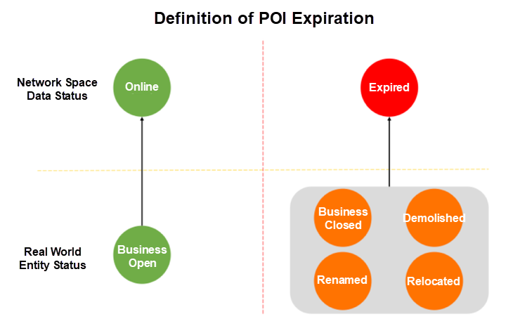
However, onsite data collection is inefficient and costly. This makes it particularly critical for us to adopt data mining algorithms, and especially time series models that are capable of handling massive volumes of data, to improve POI data recency.
The detection of expired POI records can be abstracted as a binary classification problem with skewed data. We based the project on multi-source trend features and introduced the attributes and state-level characteristics of high-dimensional sparse data to build a mixture model that met our operational needs.
This article examines the challenges related to the application of deep learning as an important tool in improving AMAP performance and discusses the feasibility of proposed solutions.
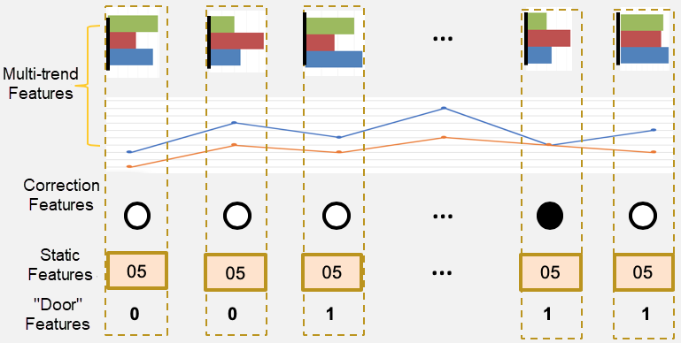
The key aim of expired POI mining is the ability to perceive and observe changes that occur after a POI expires, which is generally a drop in POI activity, and then process the data accordingly. Therefore, the key to building a high-performance time series model is constructing a framework of related features, to which we added some non-sequential features for auxiliary correction.
We correlated the POIs with several information sources and compiled the correlations into monthly statistics to use as model inputs. For the window size, we used sequences that spanned over two years in length to train the model and minimize the effect of periodic fluctuations.
We introduced the first auxiliary feature in order to leverage the manually verified historical datasets. We constructed a one-hot vector of the sequence length and then marked the month when the POI has last identified as existent with one and the rest with zero. A manually verified POI has a low risk of expiration close to the verification period. If verification was performed after the data trend turns downwards, this trend is unlikely to represent the expiration of a POI.
Our survey found that the likelihood of expiration varied for different types of POIs. For example, the rates for foodservice and lifestyle services POIs are high, while other POIs, such as place names and bus stops, are much less likely to expire. Therefore, we constructed the industry type numbers as a vector of the same sequence length and used it as the second auxiliary feature.
We constructed the third auxiliary feature while working on a missed recall issue that occurred during operation analysis. We noticed that, for many newly created POIs, the duration between the time when they were recorded in our system and the current time was shorter than the sequence length. This meant that the initial part of the trend measures for these POIs was simply 0 and had no statistical value. This could hide an actual downward trend later in the period, resulting in potential misjudgments. We devised two solutions for this issue.
The first was to deploy a dynamic window for Recurrent Neural Network (RNN) models to enable partial sequence capture for only the time since POI creation and use the result as the model input.
The second was to add a "gate" as a one-dimensional feature while maintaining the sequence length and specify the values before POI creation as zero, and the values after this time as one. The following is an example.
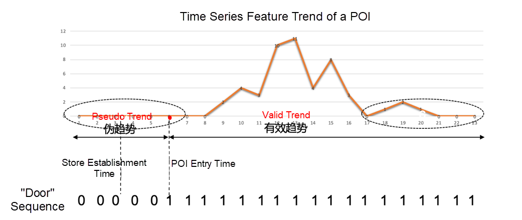
The first approach captures data only after POIs are entered into the database. However, since we do not know when the businesses represented by these POI were actually established, it is possible that some information could be lost. The "gate" method, on the other hand, balances information integrity with a specified high-confidence interval, and so we applied the second approach in our project. The following diagram demonstrates a mix of features.
Recurrent Neural Network (RNN) models deliver outstanding characterization performance and have long been the preferred choice for sequence modeling. In this project, we used an RNN variant: long short term memory (LSTM) networks.
Based on the aforementioned sequential and auxiliary features, we used multiple LSTM layers to construct the first version of the RNN model for expired data mining. The architecture of the model is described in the following diagram. The main logic is to first align the features in chronological order and use them as inputs for the deep LSTM network. We used the Softmax activation function in the output layer of the network to calculate the expiration rate. The final outputs were either automatically or manually processed based on their confidence intervals. This model provides preliminary evidence for the feasibility and benefits of using RNNs in expired data mining.

AMAP ranks POIs by popularity based on the frequency of related navigation, searches, and clicks, which means that if the top-ranked results have expired, many users will have a poor experience. The goal for updating the model version 2.0 was to improve its performance in detecting expired POIs among top results.
We discovered that the data distribution of the top-ranked POIs was very dissimilar to that of the lowest-ranked ones. Specifically, a large amount of data was available for the top POIs, with only a few POIs identified as zero, whereas the data values for the lowest-ranked POIs were sparsely distributed, and the data values for some months were lower than ten. In order to mine data with better precision, we developed an RNN model specifically for the top POIs.
We also applied padding techniques for differently ranked POIs to balance the features. For the top-ranked POIs, we substituted zero for null values to prevent interference. For the lowest-ranked POIs, we inserted values to maintain balance. These values were acquired by weighting the normalized data of other dimensions.

The 2.0 model provides improved recall for both the highest- and lowest-ranked POIs and significantly improved automation for the top POIs.
Even though the RNN model fully exploits the sequential features, the lack of feature richness still prevented us from taking automation a step further. Therefore, the major objective of this phase was to update the model through the integration of information from multiple sources. The integrated information mainly included non-sequential static information and information concerning new sequential features.
We used Wide and Deep learning as our main source of inspiration during the update and innovated on this basis. First, we encapsulated the existing RNN model as the Deep module and combined it with a Wide module. This was equivalent to rebuilding a mixture model, which required model integration in the structural dimension. Second, since we had both time-series information for the Deep module and real-time status information for the Wide module, we needed to integrate this information in the time dimension. Finally, the Wide module contained a large number of non-quantifiable or non-comparable features that needed to be encoded for characterization, which required data integration in the attribute dimension.
Feature Encoding
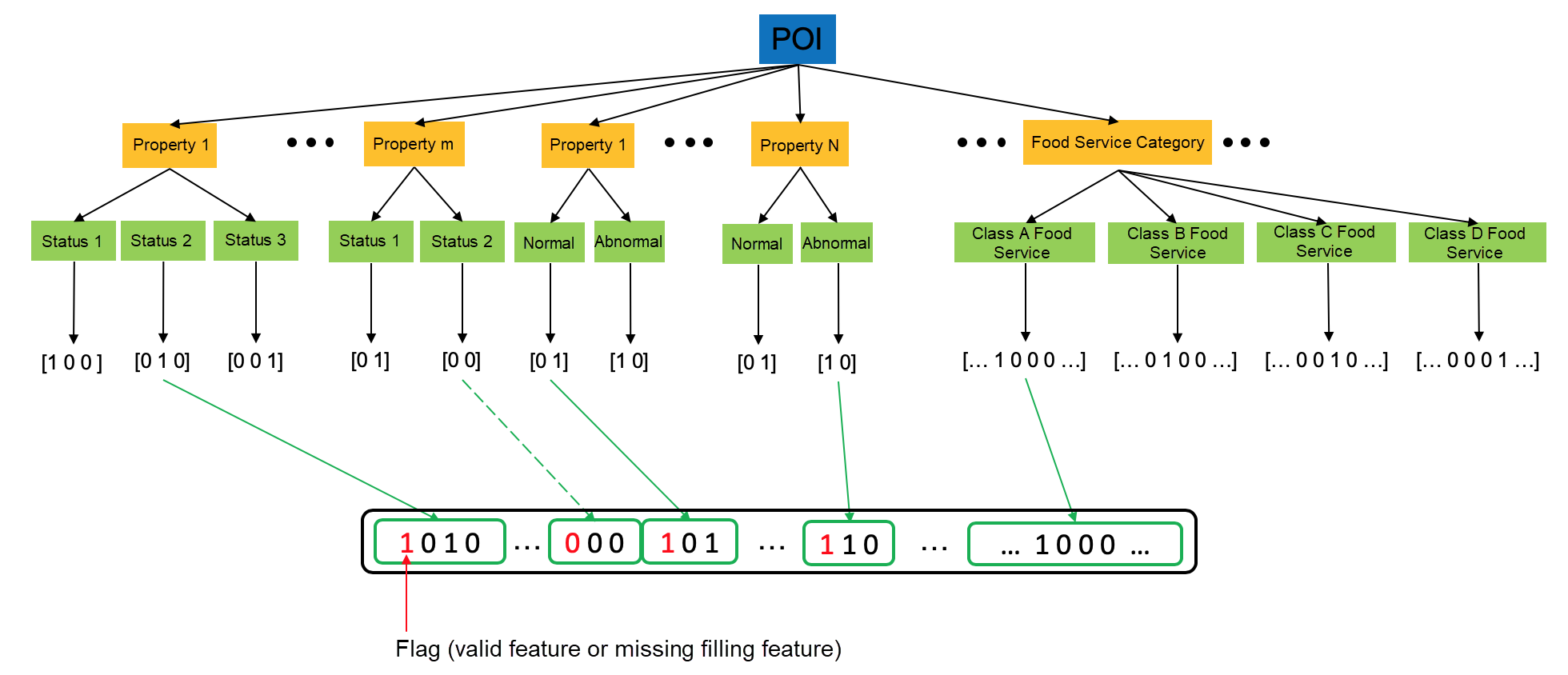
We built the Wide module with the encoded non-sequential features. This involved three main feature types: attribute, status, and business type.
Considering that some POIs were missing certain attributes, we used the first bit in the code as a flag to indicate whether the feature existed, followed by the attribute types after one-hot encoding. For status features, there was also a flag indicating whether the feature was missing, followed by the latest status type after one-hot encoding. Since different business types had different expiration rates, we used the business type as the third feature after one-hot encoding. Finally, each feature code was connected sequentially to form a high-dimensional sparse vector. The feature encoding process is shown in the following figure.
Feature Coupling
Now that the features were ready for further processing, feature coupling and model training became the most essential tasks. The features were coupled in the layer before the SoftMax output. For the RNN structure in the Deep module, the latest hidden layer was coupled. For the high-dimension sparse vector in the Wide module, we used a fully-connected network to reduce the dimensionality and obtain the hidden layer of the Wide module. Then, we connected these two hidden layers and exported the results to SoftMax to calculate the expiration rate.
We trained the model on synchronous inputs of the Wide and Deep features and balanced their weights by adjusting the dimensions of the coupled hidden layers. The structure of the Wide and LSTM model for expiration mining is shown in the following figure.
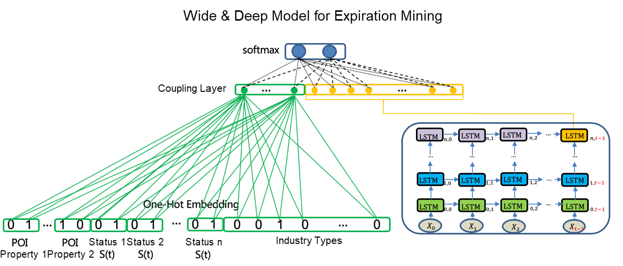
The model had been through multiple updates and optimization before it was put into production. It has become a widely-applied comprehensive model in the field of expired data mining with outstanding problem-solving performance.
The development of basic features continued as we updated the model. However, we were faced with a problem. We found huge gaps when attempting to match the long sequence features with the newly-created short and multidimensional sequence features by time order.
Using padding techniques for such large-scale feature loss across many dimensions might be counterproductive, so we took piecemeal measures instead. We built two RNN modules and put the long sequences without new features into the long RNN module, and put the short sequences with new features into the short RNN module. Then, we coupled the hidden layers of the two modules with the Wide module to get the Wide and Dual-RNN model. The structure of the Wide and Dual-RNN model is illustrated in the following diagram.
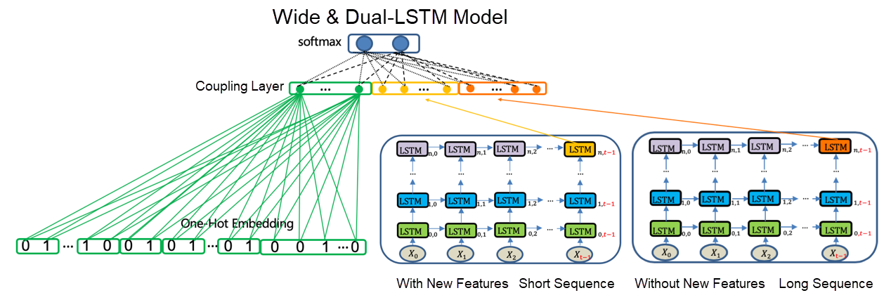
The dual-RNN structure integrated new features with the existing model and improved the judgment accuracy, but its complexity slowed down calculation. Therefore, we decided to use a more flexible time series model, temporal convolutional network (TCN).
TCN was a good choice for time series modeling. First, the convolutions in the architecture are causal, meaning that there is no information "leakage" from the future to the past. Second, it takes a sequence of any length and map it to an output sequence of a fixed length. In addition, it uses residual modules and dilated convolutions to build long-term dependencies.
In terms of performance, TCN represents time series as vectors for parallel computing. This makes it much faster than RNN's sequential calculation. Moreover, TCN accepts extended one-dimensional sequences as inputs and prevents time-specific sequence alignment. For this reason, we verified the efficiency of Wide and Deep learning and performed the following operations to update the RNN structure in the Deep module to TCN.
First, we flattened the input features to connect the time series of each dimension in an end-to-end in order to form a long vector to use as the input. In this way, the long and short features were effectively integrated.

Second, we used the attention mechanism of the sequence dimension to optimize the output structure. The key point was not to read only the concentrations of the latent vectors at the last node of the sequence but to weight the latent vector information of all sequence nodes and obtain the summarized latent vector information. In this way, the learning results of all nodes could be fully utilized.
Finally, we coupled the latent vectors generated from the Attention-TCN step with the hidden layers of the Wide module and obtained the Wide and Attention-TCN model, whose structure is shown in the following figure.
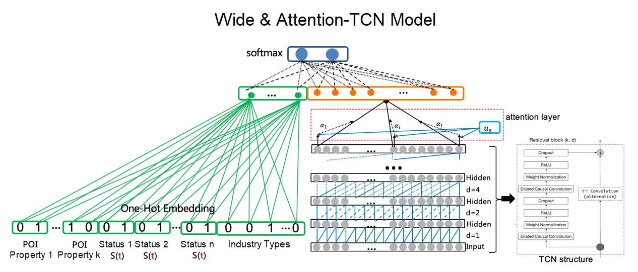
The performance of the new model was further improved with the introduction of the new lightweight TCN time series model and the attention mechanism. However, the tuning process was more complicated than for the RNN. After multiple rounds of parameter tuning and structure optimization, the computing speed and recall of the final version increased remarkably compared with the Wide and Dual-LSTM version.
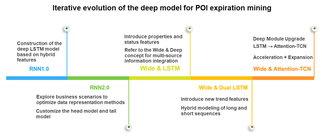
The implementation of deep learning for expired data mining is an iterative process of evaluation that combines stages of exploration, summarization, optimization, and verification. Not only did we achieve our goal of enhancing our expired data mining capabilities, but we also gained experience in feature extension, feature construction, and model structure optimization. The keys to our success in performance improvement were rich and reliable features, suitable characterization methods, and scenario-compliant model structures.
The current model summarizes macro rules based on information and trends and can likewise be used to calculate the rate of expiration for POIs. However, in real-life applications, when considering the possibility of POI expiration, we have to take other factors, such as the specific geographical location, business conditions, and nearby competitors, into account. In the future, we will explore overall regularities and individual differences to achieve more refined detection.
AMAP on the Go: Effective Ways to Respond to Customer Feedback
Exploration and Practice of Deep Learning Application in AMAP ETA
Alibaba Clouder - June 17, 2020
amap_tech - October 29, 2020
amap_tech - November 11, 2019
amap_tech - December 4, 2019
Tim Chen - May 22, 2019
Alibaba Cloud Community - August 22, 2025
 Platform For AI
A platform that provides enterprise-level data modeling services based on machine learning algorithms to quickly meet your needs for data-driven operations.
Learn More Epidemic Prediction Solution
This technology can be used to predict the spread of COVID-19 and help decision makers evaluate the impact of various prevention and control measures on the development of the epidemic.
Learn More Big Data Consulting for Data Technology Solution
Alibaba Cloud provides big data consulting services to help enterprises leverage advanced data technology.
Learn More Big Data Consulting Services for Retail Solution
Alibaba Cloud experts provide retailers with a lightweight and customized big data consulting service to help you assess your big data maturity and plan your big data journey.
Learn MoreMore Posts by amap_tech