With the popularization of mobile devices, more and more business data includes spatial data such as FEED information for a mobile phone user, and Internet of Things, Internet of Vehicles, meteorological sensor data, animal source data, and a variety of tracking data.
Data is measured in the following dimensions:
Data pivoting is crucial for company BI, analysts, and daily operation. It used be subject to a combination of business and temporal characteristics, but now we also do spatial pivoting (for example, pivoting near a certain point over a certain period of time, pivoting for a certain province, or pivoting over Northern latitudes.)
Precomputation, real-time computation, and StreamCompute are all critical to real-time pivoting.
Data in the examples above does not include a spatial element. In this article we will examine database design and DEMO for data pivoting when multiple dimensions like space, time, and business characteristics are in play.
Let's look at an example of spatial and temporal data pivoting.
Sensors are installed on Didis, taxis, buses, coaches, and hazardous chemical vehicles. These sensors are continuously generating and reporting data as their locations move along with the vehicles.
At the same time, there are also static sensors uploading and reporting data.
There are 3 data structures. Different reporting modes correspond to different structures.
1. Single data report mode
table
(
  sid int, -- the sensor ID
  pos geometry, -- the sensor position
  ts timestamp, -- the time
  val1 int, -- the value of property 1 detected by the sensor
  val2 float, -- the value of property 2 detected by the sensor
  val3 text -- the value of property 3 detected by the sensor
  ......
)
2. Batch report mode: aggregated details (one record includes multiple values)
table
(
  sid int, -- the sensor ID
  pos geometry[], -- the sensor position
  ts timestamp[], -- the array of time
  val1 int, -- the array of values for property 1 detected by the sensor
  val2 float[], -- the array of values for property 2 detected by the sensor
  val3 text[] -- the array of values for property 3 detected by the sensor
  ......
)
3. Batch report mode: package details in JSON format
table
(
  sid int, -- the sensor ID
  info jsonb -- Batch packaging of data {k1: {pos:val, ts:val, val1:val, val2:val, ...}, k2: {}, k3: {}, ....}
) Two data pivoting architecture designs are available: one is real-time bare calculation, which is aggressive and requires more computing capability, but is appropriate for situations when a model cannot be created.
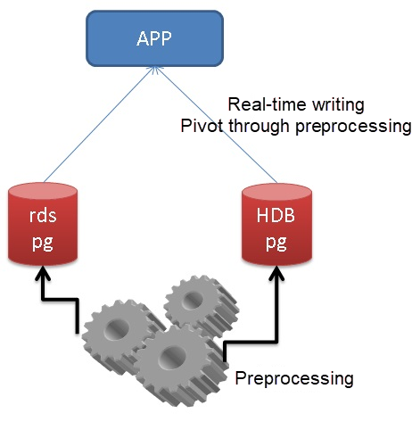
The other architecture can be used when you can create a model. Pretreatment reduces costs and response time is improved.
See below:
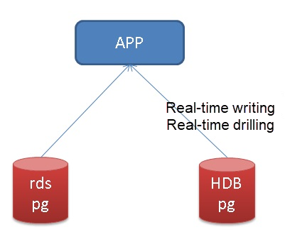
I. Real-time architecture
Real-time mode, which involves drawing statistics from query results. The speed of query response depends on the cluster's computational ability. Heavy investment is generally required if you want to keep response speeds high.
II. Pre-treatment architecture
Many pre-treatment methods are available: StreamCompute, T+N scheduling, and lambda scheduling.
1. Stream processing
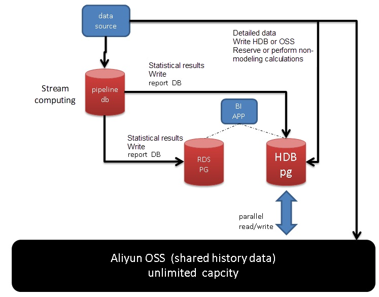
PostgreSQL's plug-in PipelineDB (will be converted to a plug-in in July) can be selected for StreamCompute. StreamCompute supports PostgreSQL's built-in TTL, sliding window, estimated value statistics, aggregation statistics function, etc. Performance is good, as a single machine has a processing speed of 1 million lines/s.
The data source is written into PipelineDB for StreamCompute. If StreamCompute results (for example, the statistics dimension is day, 7 is set for TTL, and the statistics result on the previous day is written into the report library RDS PG or HDB PG every day) and detailed data of the data source needs to be reserved, you can write them into HDB PG or OSS.
This architecture design can achieve millisecond-level response times in situations where a model can be created. HDB PG's parallel computing capability can also be applied to situations where models cannot be created (real-time calculations have to be performed in detail) for faster response times.
2. T+N scheduling
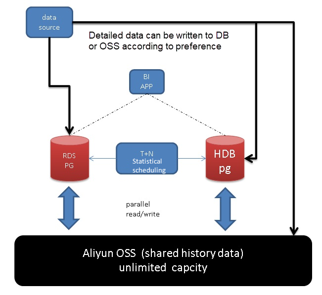
This is actually a common report system methodology. For example, detailed data is imported to the database or OSS in the early hours of the day, and a report is generated based on the model.
3. Lambda scheduling
T+N scheduling is only applicable when changing the StreamCompute node into HDB PG or RDS PG, incrementally making statistics of modeling data, and merging the statistics result through FUNCIONT and job scheduling.
Partition rules are used in data nodes. A rule should take into account the method by which the data is queried, for example search or query based on temporal or spatial ranges, in which case we provide two partition dimensions.
Both PostgreSQL and HDB support multi-level partitioning, so we can make a multi-level partition based on the two dimensions.
   [ PARTITION BY partition_type (column)
       [ SUBPARTITION BY partition_type (column) ]
          [ SUBPARTITION TEMPLATE ( template_spec ) ]
       [...]
    ( partition_spec )
        | [ SUBPARTITION BY partition_type (column) ]
          [...]
    ( partition_spec
      [ ( subpartition_spec
           [(...)]
         ) ]
    )


where partition_type is:
    LIST
  | RANGE


where partition_specification is:
partition_element [, ...]

and partition_element is:
   DEFAULT PARTITION name
  | [PARTITION name] VALUES (list_value [,...] )
  | [PARTITION name]
     START ([datatype] 'start_value') [INCLUSIVE | EXCLUSIVE]
     [ END ([datatype] 'end_value') [INCLUSIVE | EXCLUSIVE] ]
     [ EVERY ([datatype] [number | INTERVAL] 'interval_value') ]
  | [PARTITION name]
     END ([datatype] 'end_value') [INCLUSIVE | EXCLUSIVE]
     [ EVERY ([datatype] [number | INTERVAL] 'interval_value') ]
[ WITH ( partition_storage_parameter=value [, ... ] ) ]
[column_reference_storage_directive [, ...] ]


where subpartition_spec or template_spec is:
subpartition_element [, ...]
and subpartition_element is:
   DEFAULT SUBPARTITION name
  | [SUBPARTITION name] VALUES (list_value [,...] )
  | [SUBPARTITION name]
     START ([datatype] 'start_value') [INCLUSIVE | EXCLUSIVE]
     [ END ([datatype] 'end_value') [INCLUSIVE | EXCLUSIVE] ]
     [ EVERY ([datatype] [number | INTERVAL] 'interval_value') ]
  | [SUBPARTITION name]
     END ([datatype] 'end_value') [INCLUSIVE | EXCLUSIVE]
     [ EVERY ([datatype] [number | INTERVAL] 'interval_value') ]
[ WITH ( partition_storage_parameter=value [, ... ] ) ]
[column_reference_storage_directive [, ...] ]
[ TABLESPACE tablespace ]
1. For example, a partition based on temporal ranges will be recreated every day.
2. Geohash range. Geohash is a code value representing a box composed of longitude and latitude coordinates. The length of the code determines its precision (size). Code prefixes of adjacent boxes are identical. Therefore, you can code within the range by using geohash.
For example, if you need to search data over a certain period of time, you can use the partition rule and pick up the corresponding partitions to narrow down the query range.
If you need to search data within a certain spatial range, you can make the partition based on the geohash range and query the corresponding partitions to narrow down the query range.
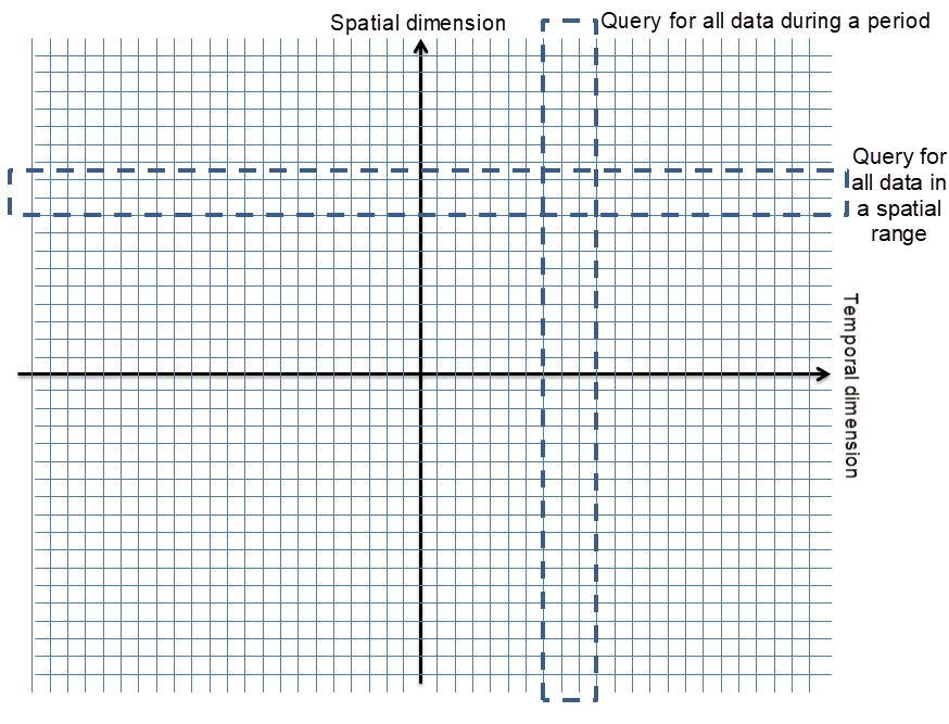
HDB supports both geohash and geometry. You can create a GIST spatial index on geometry. KNN search is supported for spatial indexes (precise retrieval is irrelevant to the box).
A distribution determines how data is distributed across multiple node layers. It should not be the same as the partition rule. We can either use a random distribution rule or base it on a business related data field. Either way, we need to take data skew into consideration.
1. Random distribution: data is randomly written into different nodes to ensure uniformity. But you need to invoke all data nodes during each query. Data re-distribution will be involved for JOIN operations.
2. Business ID: distribution by business ID. When querying by the business ID, you only need to invoke the data node where the corresponding business ID is located. But you need to consider data skew. For example, data may not be uniform if a business ID contains a large amount of data.
PS: (consistent HASH solves the issue of non-uniformity in data distribution.)
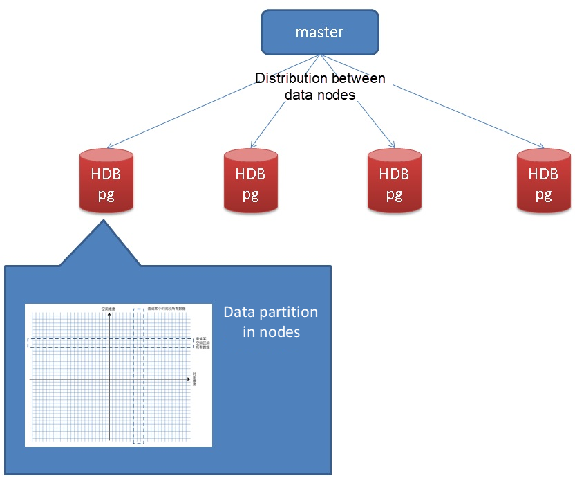
Pre-calculation is a method by which pivoting response time can be significantly reduced in situations where modeling can be used.
In addition to precomputation of business indicators, precomputation of temporal and spatial dimensions is also common.
There is a commonality for statistics. Statistics are made by grouping, for example by time (hour, day, month, year, etc.), and space (administrative region, box, geohash, grid, etc.).
For example, business reports can be queried by day, month, and year. So we can precompute by day.
Multi-dimensional pivoting is done with the GROUPING SETS statement.
insert into result
select date(crt_time),col1,col2,col3,...,agg_func1(),agg_func2(),...
from table
  where crt_time between ? and ?
group by date(crt_time),GROUPING SETS(col1,col2,col3,...); In the movie Interstellar, the protagonist creates a five-dimensional space which allows him to move freely across time.

Data pivoting can operate on a similar concept. You may need to query statistics within any time window in past records.
For example, you may have to query statistics 30 minutes before and after 27 June 2017 13:50:00.
There are two methods by which sliding window can be implemented:
1. Non-precomputed: involves generating statistics directly based on data details.
2. If the sliding window requires precomputation, we need to calculate our statistics at a finer granularity. For example, if the window size is 1h, then we need to calculate in increments smaller than 1h. For example, if we calculate down to the half hour, then when we query the sliding window, then the statistical result will be derived from a second round of calculation performed on the results of the first calculation on our half hour data.
Sliding window is also implemented this way in PipelineDB.
http://docs.pipelinedb.com/sliding-windows.html
In order to perform precomputation on the spatial dimension, we need to group the spatial data based on business requirements and on the spatial data pivoting.
Example
1. Business requirements are counted based on the district-level administrative region. Therefore, we can implement pre-calculation based on the district-level administrative region (picture taken from the Internet).
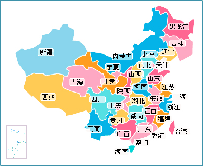
First, functional support must be provided for translating the administrative region ID. Second, return the ID of the administrative region where the longitude and latitude coordinates are located.
A traditional method is to denote the geometry of an administrative region by a table, and use a GIST index to quickly return the geometry of the region based on the longitude and latitude values.
table (
  ID int, -- the ID of the administrative region
  bb geometry -- the geometry of the administrative region
)

create or replace function get_id(pos geometry) returns int as
$$

  select id from table where bb && pos limit 1;

$$
 language sql strict immutable;
Statistics
insert into result
select get_id(pos),col1,col2,col3,...,agg_func1(),agg_func2(),...
from table
  where crt_time between ? and ?
  group by get_id(pos),GROUPING SETS(col1,col2,col3,...);
2. Calculate by geohash prefix. For example, removing a 5-bit hash, and aggregating it (calculate the geohash value of the longitude and latitude through the PostGIS ST_GeoHash() function).
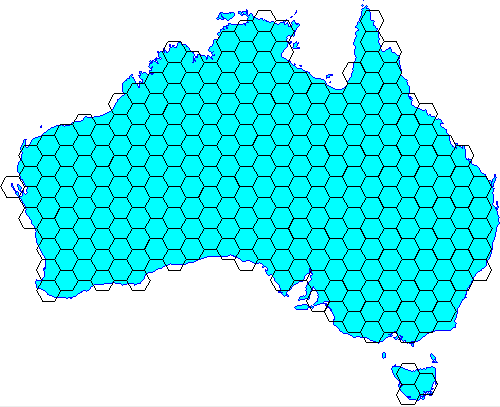
insert into result
select ST_GeoHash(pos,5),col1,col2,col3,...,agg_func1(),agg_func2(),...
from table
  where crt_time between ? and ?
  group by ST_GeoHash(pos,5),GROUPING SETS(col1,col2,col3,...);
Geohash precision is as follows:
so one symbol (letters or digits) is base 32 (8 bits) Each first bit is used for high or low window,
then subsequent bits divide the precision by 2.

(so divide by 8 in the best case) but there is an alternance between lat and long precision,
so it ends up dividing by 4 and 8 alternatively.

#   km
1   ±2500
2   ±630
3   ±78
4   ±20
5   ±2.4
6   ±0.61
7   ±0.076
8   ±0.019
9   ±0.0024
10  ±0.00060
11  ±0.000074

Note that, as mentioned on the Wiki page, those values come from a location near the equator,
where a degree has nearly the same lenght in X and Y.

For a more accurate information, you should start from the lat and long errors,
and compute the km precision along X-axis based on the latitude of your position. Implementation of sliding spatial sliding windows is similar to that of temporal sliding windows. For example, we can calculate an 8 bit geohash code, and code by a 5-bit geohash to perform secondary aggregated pivoting.
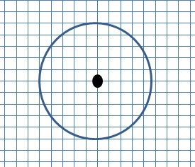
A certain degree of distortion is inevitable when calculating statistics for spatial and temporal sliding windows. (because it is impossible for the boundary to be totally clear).
If this is a concern, you can consider real-time calculation.
Precomputation of business dimensions is similar to that of temporal and spatial dimensions. It will not be described here.
select sum,avg,count,min,max,hll,....
  from result
where
  ts =
  and val1 =
and ...; Secondary aggregation is required for sliding made through precomputation. Follow these steps:
sum = sum(sum)
count = sum(count)
min = min(min)
max = max(max)
avg = sum(sum)/sum(count)
hll = hll_union_agg(hll)
select sum(sum),sum(count),hll_union_agg(hll),...
  from result
where
  ts between ? and ?
  and val1 =
and ...; select sum,avg,count,min,max,hll,....
from result
where
loc_id = ?
and val1 =
and ...; sum = sum(sum)
count = sum(count)
min = min(min)
max = max(max)
avg = sum(sum)/sum(count)
hll = hll_union_agg(hll)
select sum(sum), sum(count), hll_union_agg(hll), ...
from result
where
substring(geohash_val, 1, 5) = ?
and val1 =
and ...; If you don't need to query specific details, or frequently query only a few details with low delay, then you don't need to enter detailed data into the database. Rather you can just import it to OSS.
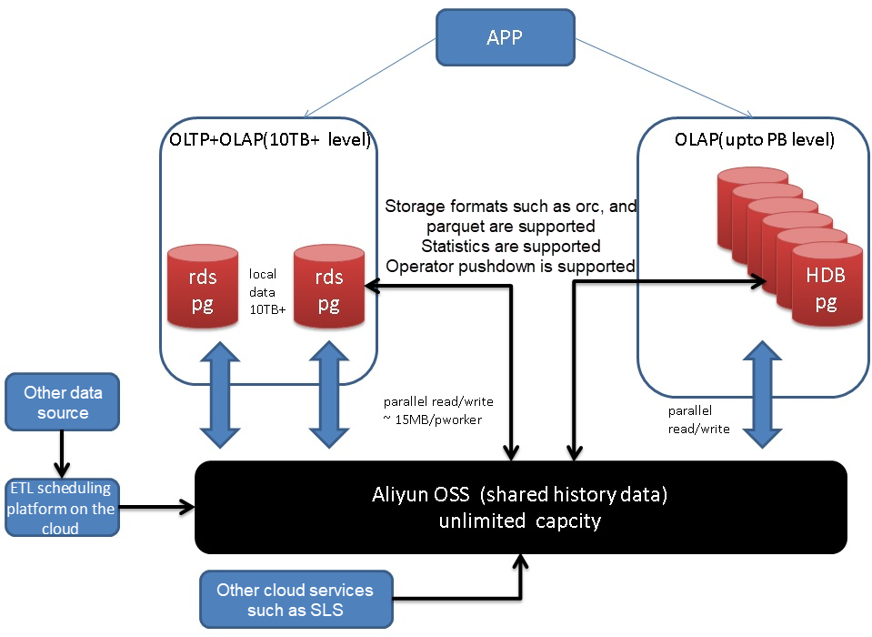
You can use RDS PG or HDB PG to concurrently access OSS and implement real-time pivoting or precomputation.
StreamCompute mode: create a stream based on the data structure, create a statistics view for the stream, activate the statistics view, write the data into the database in real time, and perform real-time statistics on flowing data in the database to generate statistics results.
If too many statistics results are provided, we can use TTL statistics view to regularly transfer them to HDB.
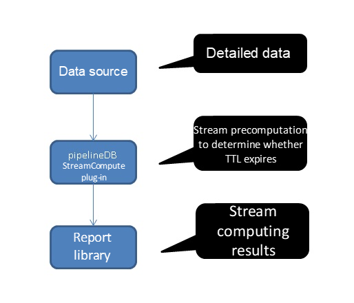
Example
Define stream
create stream s1 (
  sid int, -- the sensor ID
  pos geometry, -- the sensor position
  ts timestamp, -- the time
  val1 int, -- the value of property 1 detected by the sensor
  val2 float, -- the value of property 2 detected by the sensor
  val3 text -- the value of property 3 detected by the sensor
  ......
);
Define TTL statistics view and maintain for one week
CREATE CONTINUOUS VIEW v1 WITH (ttl = '7 day', ttl_column = 'crt_time') AS
select date(crt_time) crt_time,col1,col2,col3,...,agg_func1(),agg_func2(),...
from table
  group by date(crt_time),GROUPING SETS(col1,col2,col3,...);
Activate statistics view
ACTIVATE v1; Regular data transfer
insert into result
  select * from v1 where crt_time = 'yesterday';
Data pivoting
select * from result ....; 1. Why don't we create a composite index of time and space fields?
If I need to query data for a certain point in the neighboring N kilometers at a certain time interval, how can I quickly locate the target detailed data?
You need to quickly converge to one dimension when creating an index in the actual and spatial dimensions. If you want to converge to another dimension, you need to obtain a tuple through heap, then recheck and filter.
Why don't we create a composite index of time and space fields? Because queries are continuous, scanning all index entries in drive columns is required for the composite index.
Query efficiency for equivalent drive columns is very high using the composite index.
It is recommended that the partition be used for data queries of temporal and spatial dimensions. Partition is the most effective method of narrowing down the data range.
It is recommended that geohash range partition be used for the partition of the spatial dimension.
2. Precomputation is the core of millisecond-level pivoting on any dimension.
3. The data estimation type is HLL. It helps you quickly query the number of unique and newly added values.
4. If you need to aggregate detailed values, you can store them using fields like array and JSONB.
5. Alibaba Cloud RDS PG, HDB for PG, OSS, StreamCompute plug-in, cloud ETL scheduling task service provide a comprehensive big data real-time calculation solution for millisecond-level data pivoting of any temporal or spatial dimension.
6. For spatial data, in addition to using the GiST index, we also provided a more cost-effective index, the BRIN index, which is excellent for filtering data structured by st_geohash.
Use Cases for Millisecond-Level Massive Multi-Dimensional Data Pivoting on PostgreSQL/GPDB
digoal - June 26, 2019
Alibaba Clouder - September 27, 2019
Alibaba Cloud Storage - March 28, 2019
Alibaba Clouder - July 7, 2020
digoal - January 18, 2021
Alibaba Cloud Community - January 9, 2026
 PolarDB for PostgreSQL
Alibaba Cloud PolarDB for PostgreSQL is an in-house relational database service 100% compatible with PostgreSQL and highly compatible with the Oracle syntax.
Learn More Time Series Database (TSDB)
TSDB is a stable, reliable, and cost-effective online high-performance time series database service.
Learn More Big Data Consulting for Data Technology Solution
Alibaba Cloud provides big data consulting services to help enterprises leverage advanced data technology.
Learn More Cloud Migration Solution
Secure and easy solutions for moving you workloads to the cloud
Learn MoreMore Posts by digoal