Platform For AI：Responsible AI-公平性分析

Sklearn

from sklearn.linear_model import LogisticRegression

# 建立羅吉斯迴歸模型
sk_model = LogisticRegression(solver='liblinear', fit_intercept=True)
# 模型訓練
sk_model.fit(X_train, y_train)

PyTorch

import torch
import torch.nn as nn
import torch.optim as optim

# 定義羅吉斯迴歸模型
class LogisticRegression(nn.Module):
    def __init__(self, input_size):
        super(LogisticRegression, self).__init__()
        self.linear = nn.Linear(input_size, 1)

    def forward(self, x):
        outputs = torch.sigmoid(self.linear(x))
        return outputs

# 執行個體化模型
input_size = X_train.shape[1]
pt_model = LogisticRegression(input_size)

# 損失函數和最佳化器
criterion = nn.BCELoss()
optimizer = optim.SGD(pt_model.parameters(), lr=5e-5)

# 訓練模型
num_epochs = 1
X_train_pt = X_train
y_train_pt = y_train
for epoch in range(num_epochs):
    # 前向傳播
    # DataFrame 轉換為 Tensor
    if isinstance(X_train_pt, pd.DataFrame):
        X_train_pt = torch.tensor(X_train_pt.values)
        X_train_pt = X_train_pt.float()
    outputs = pt_model(X_train_pt)
    outputs = outputs.squeeze()
    # ndarray 轉換為 Tensor
    if isinstance(y_train_pt, np.ndarray):
        y_train_pt = torch.from_numpy(y_train_pt)
        y_train_pt = y_train_pt.float()
    loss = criterion(outputs, y_train_pt)

    # 反向傳播和最佳化
    optimizer.zero_grad()
    loss.backward()
    optimizer.step()

TensorFlow

import tensorflow as tf
from tensorflow.keras import layers

# 定義羅吉斯迴歸模型
tf_model = tf.keras.Sequential([
    layers.Dense(units=1, input_shape=(X_train.shape[-1],), activation='sigmoid')
])

# 編譯模型，使用二元交叉熵損失和隨機梯度下降最佳化器
tf_model.compile(optimizer='sgd', loss='binary_crossentropy', metrics=['accuracy'])

# 訓練模型
tf_model.fit(X_train, y_train, epochs=1, batch_size=32, verbose=0)

Sklearn

from raiwidgets import FairnessDashboard
import os
from urllib.parse import urlparse
# 根據測試資料集進行預測結果
y_pred_sk = sk_model.predict(X_test)

# 使用 responsible-ai-toolbox  計算每個敏感群體的資料資訊
metric_frame_sk = FairnessDashboard(sensitive_features=sensitive_features_test,
                  y_true=y_test,
                  y_pred=y_pred_sk, locale = 'zh-Hans')

# 設定URL跳轉連結
metric_frame_sk.config['baseUrl'] =  'https://{}-proxy-{}.dsw-gateway-{}.data.aliyun.com'.format(
    os.environ.get('JUPYTER_NAME').replace("dsw-",""),
    urlparse(metric_frame_sk.config['baseUrl']).port,
    os.environ.get('dsw_region') )
print(metric_frame_sk.config['baseUrl'])

PyTorch

from raiwidgets import FairnessDashboard
import torch
import os
from urllib.parse import urlparse
# 測試模型並評估公平性
pt_model.eval()  # 設定模型為評估模式
X_test_pt = X_test
with torch.no_grad():
    X_test_pt = torch.tensor(X_test_pt.values)
    X_test_pt = X_test_pt.float()
    y_pred_pt = pt_model(X_test_pt).numpy()

# 使用 responsible-ai-toolbox  計算每個敏感群體的資料資訊
metric_frame_pt = FairnessDashboard(sensitive_features=sensitive_features_test,
                           y_true=y_test,
                           y_pred=y_pred_pt.flatten().round(),locale='zh-Hans')

# 設定URL跳轉連結
metric_frame_pt.config['baseUrl'] =  'https://{}-proxy-{}.dsw-gateway-{}.data.aliyun.com'.format(
    os.environ.get('JUPYTER_NAME').replace("dsw-",""),
    urlparse(metric_frame_pt.config['baseUrl']).port,
    os.environ.get('dsw_region') )
print(metric_frame_pt.config['baseUrl'])

TensorFlow

from raiwidgets import FairnessDashboard
import os
from urllib.parse import urlparse
# 測試模型並評估公平性
y_pred_tf = tf_model.predict(X_test).flatten()

# 使用 responsible-ai-toolbox  計算每個敏感群體的資料資訊
metric_frame_tf = FairnessDashboard(
                           sensitive_features=sensitive_features_test,
                           y_true=y_test,
                           y_pred=y_pred_tf.round(),locale='zh-Hans')

# 設定URL跳轉連結
metric_frame_tf.config['baseUrl'] =  'https://{}-proxy-{}.dsw-gateway-{}.data.aliyun.com'.format(
    os.environ.get('JUPYTER_NAME').replace("dsw-",""),
    urlparse(metric_frame_tf.config['baseUrl']).port,
    os.environ.get('dsw_region') )
print(metric_frame_tf.config['baseUrl'])

敏感特徵為“sex”

• 敏感特徵：sex

• 效能指標：Accuracy

• 公平性指標：Demographic parity difference

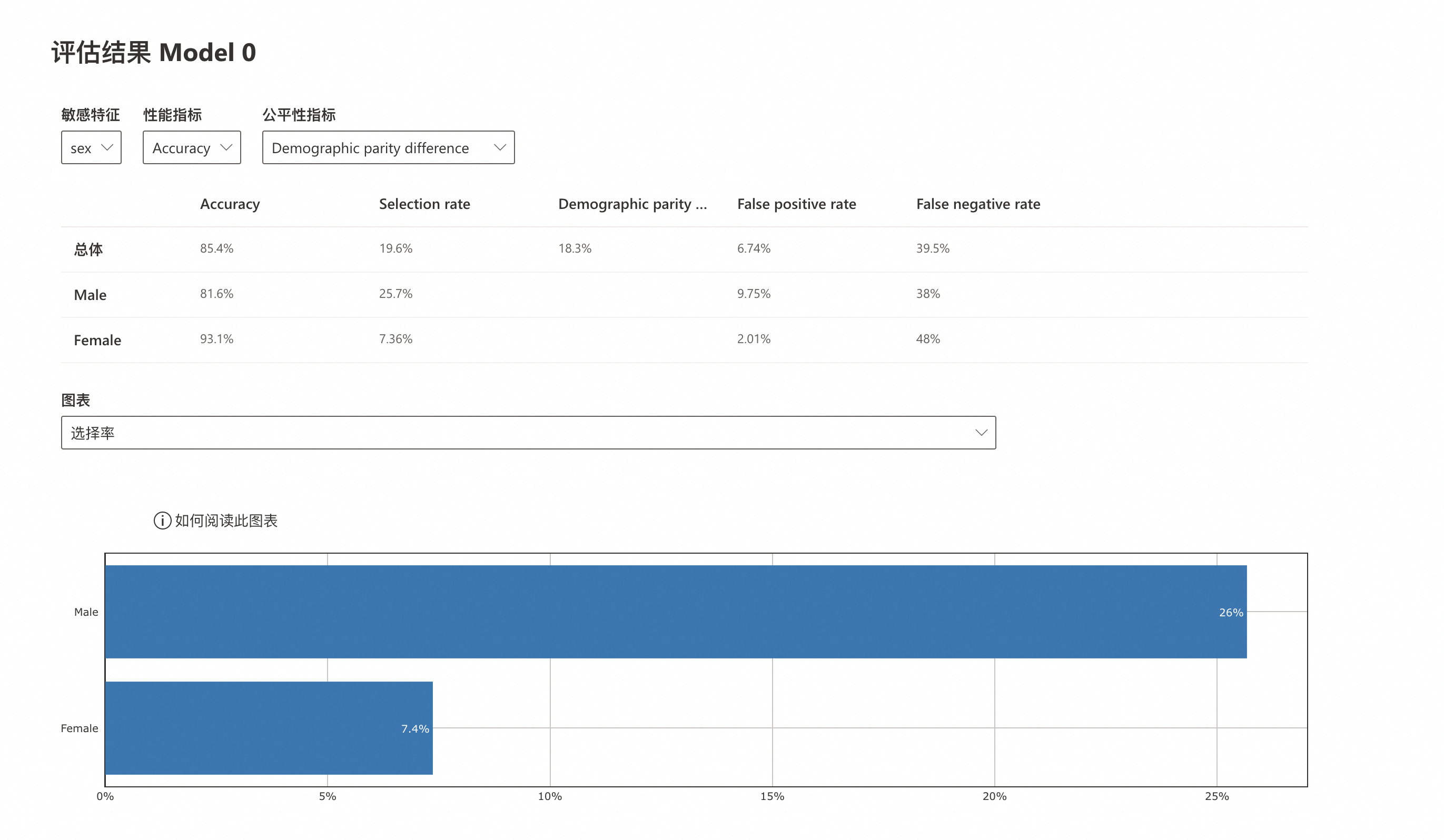
• Accuracy：精確度，是指模型正確預測的樣本數佔總樣本數的比例。模型輸出男性個人年度營收的準確度（81.6%）低於女性個人年度營收的準確度（93.1%），但是兩者的準確度與模型總體準確度（85.4%）都比較接近。

• Selection rate：選擇率，是指模型輸出“好”的目標變數的機率，這裡“好”的目標變數是個人年度營收>50K。模型輸出男性個人年度營收>50K的機率（25.7%）大於女性個人年度營收>50K的機率（7.36%），並且模型輸出女性個人年度營收>50K的機率（7.36%）遠低於個人年度營收>50K的總體機率（19.6%）。

• Demographic parity difference：人口統計公平性差異，是指不同受保護群體之間，在指定的敏感屬性下獲得積極預測結果的機率差異。這個值越接近0，意味著群體間的偏差越小。模型總體的人口統計公平性差異為18.3%。

敏感特徵為“race”

• 敏感特徵：race

• 效能指標：Accuracy

• 公平性指標：Demographic parity difference

• Accuracy：精確度，是指模型正確預測的樣本數佔總樣本數的比例。模型輸出“White”和“Asian-Pac-Islander”個人年度營收的準確度（84.9%和79.1%）低於“Black”、“Other”和“Amer-Indian-Eskimo”個人年度營收的準確度（90.9%、90.8%和91.9%），但是所有敏感特徵人群的準確度與模型總體準確度（85.4%）都比較接近。

• Selection rate：選擇率，是指模型輸出“好”的目標變數的機率，這裡“好”的目標變數是個人年度營收>50K。模型輸出“White”和“Asian-Pac-Islander”個人年度營收>50K的選擇率（21%和23.9%）大於“Black”、“Other”和“Amer-Indian-Eskimo”個人年度營收>50K的選擇率 （8.34%、10.3%和8.14%），並且“Black”、“Other”和“Amer-Indian-Eskimo”個人年度營收>50K的選擇率（8.34%、10.3%和8.14%）遠低於個人年度營收>50K的總體選擇率（19.6%）。

• Demographic parity difference：人口統計公平性差異，是指不同受保護群體之間，在指定的敏感屬性下獲得積極預測結果的機率差異。這個值越接近0，意味著群體間的偏差越小。模型總體的人口統計公平性差異為15.8%。