PAI (Platform for AI) は responsible-ai-toolbox を DSW (Data Science Workshop) に統合しており、AI モデルのバイアスを検出して修正できます。公平性分析は、モデルが性別や人種などの機密性の高い属性に基づいて不公平な予測を行っているかどうかを特定します。
基本原則
公平性分析は、AI モデルがすべてのグループを公平に扱うことを保証するのに役立ちます。基本原則は次のとおりです:
-
バイアスの回避: データとアルゴリズムのバイアスを特定して削減し、個人の特性に基づく不公平な決定を防ぎます。
-
代表性のあるデータ: すべてのユーザーグループを正確に代表する多様なデータセットを使用します。
-
透明性: 説明可能な AI 技術を使用して、ユーザーがモデルの決定を理解できるようにします。
-
継続的なモニタリング: モデルを定期的に評価し、時間とともに現れる可能性のあるバイアスを特定して修正します。
-
多様性と包括性: AI システムの設計と開発に多様な視点を取り入れます。
-
コンプライアンス: 関連する法律、規制、倫理基準に従います。
次の例では、収入予測モデル (年間収入 >50K) が性別と人種に関連するバイアスを示しているかどうかを評価します。
前提条件
-
以下の構成を持つ DSW インスタンス。詳細については、「DSW インスタンスの作成」をご参照ください。
-
推奨インスタンスタイプ: ecs.gn6v-c8g1.2xlarge
-
イメージ: tensorflow-pytorch-develop:2.14-pytorch2.1-gpu-py311-cu118-ubuntu22.04 (Python 3.9 以降)
-
サポートされているフレームワーク: Scikit-learn、PyTorch、または TensorFlow (回帰および二値分類モデル)
-
-
トレーニングデータセット。独自のデータセットを使用するか、「ステップ3」に従ってサンプルデータセットを使用できます。
-
アルゴリズムモデル。独自のモデルを使用するか、「ステップ5」に従ってサンプルモデルをトレーニングできます。
ステップ1: DSW ギャラリーノートブックを開く
-
PAI コンソールにログインします。
-
左上のコーナーで、リージョンを選択します。
-
左側のナビゲーションウィンドウで、[クイックスタート] > [ノートブックギャラリー] を選択します。Responsible AI-Fairness Analysis を検索し、[DSW で開く] をクリックします。
-
DSW インスタンスを選択し、[ノートブックを開く] をクリックします。
ステップ2: 依存関係のインストール
responsible-ai-toolbox パッケージ (raiwidgets) をインストールします:
!pip install raiwidgets==0.34.1ステップ3: データセットの読み込み
OpenML からデータセット 1590 を読み込みます:
from raiutils.common.retries import retry_function
from sklearn.datasets import fetch_openml

class FetchOpenml(object):
    def __init__(self):
        pass
    # data_id = 1590 の OpenML データセットを取得します
    def fetch(self):
        return fetch_openml(data_id=1590, as_frame=True)

fetcher = FetchOpenml()
action_name = "Dataset download"
err_msg = "Failed to download openml dataset"
max_retries = 5
retry_delay = 60
data = retry_function(fetcher.fetch, action_name, err_msg,
                      max_retries=max_retries,
                      retry_delay=retry_delay)
または、独自のデータセットを CSV 形式で読み込みます:
import pandas as pd

# 独自のデータセットを CSV 形式で読み込みます。
# pandas を使用して CSV ファイルを読み取ります。
data = pd.read_csv(filename)
ステップ4: データの前処理
特徴量変数とターゲット変数の抽出
この例では:
-
ターゲット変数 (クラス): 年間収入が 50K を超えるかどうか
-
機密性の高い特徴量: sex、race
-
その他の特徴量: age および追加の属性
特徴量変数を読み取ります:
# ターゲット変数を除いた特徴量変数を取得します。
X_raw = data.data
# ターゲット変数を除いた特徴量変数の最初の 5 行を表示します。
X_raw.head(5)
ターゲット変数の値を設定します。値「1」は収入 >50K を示し、「0」は収入 ≤50K を示します:
from sklearn.preprocessing import LabelEncoder

# ターゲット変数を二値分類ターゲットに変換します。
# data.target はターゲット変数 'class' です。
y_true = (data.target == '>50K') * 1
y_true = LabelEncoder().fit_transform(y_true)

import matplotlib.pyplot as plt
import numpy as np

# ターゲット変数の分布を表示します。
counts = np.bincount(y_true)
classes = ['<=50K', '>50K']
plt.bar(classes, counts)
機密性の高い特徴量の定義
性別と人種を機密性の高い特徴量として設定します。ツールボックスは、モデルの予測がこれらの特徴量に関してバイアスがかかっているかどうかを評価します:
# 'sex' と 'race' を機密情報として定義します。
# まず、データセットから機密情報に関連する列を選択し、`sensitive_features` という名前の新しい DataFrame を作成します。
sensitive_features = X_raw[['sex','race']]
sensitive_features.head(5)
特徴量セットから機密性の高い特徴量を削除します:
# 特徴量変数から機密性の高い特徴量を削除します。
X = X_raw.drop(labels=['sex', 'race'],axis = 1)
X.head(5)
特徴量のエンコードと標準化
ツールボックスとの互換性のためにデータを標準化します:
import pandas as pd
from sklearn.preprocessing import StandardScaler

# データをワンホットエンコードします。
X = pd.get_dummies(X)

# データセット X の特徴量を標準化 (スケーリング) します。
sc = StandardScaler()
X_scaled = sc.fit_transform(X)
X_scaled = pd.DataFrame(X_scaled, columns=X.columns)

X_scaled.head(5)
トレーニングセットとテストセットへの分割
データを 20% のテスト用に分割します:
from sklearn.model_selection import train_test_split

# 特徴量変数 X とターゲット変数 y を `test_size` の比率に従ってトレーニングセットとテストセットに分割します。
X_train, X_test, y_train, y_test = \
    train_test_split(X_scaled, y_true, test_size=0.2, random_state=0, stratify=y_true)

# 同じランダムシードを使用して、機密性の高い特徴量をトレーニングセットとテストセットに分割し、前の分割との一貫性を確保します。
sensitive_features_train, sensitive_features_test = \
    train_test_split(sensitive_features, test_size=0.2, random_state=0, stratify=y_true)
データセットのサイズを表示します:
print("Training dataset size:", len(X_train))
print("Test dataset size:", len(X_test))
インデックスをリセットします:
# DataFrame のインデックスをリセットして、インデックスエラーを回避します。
X_train = X_train.reset_index(drop=True)
sensitive_features_train = sensitive_features_train.reset_index(drop=True)
X_test = X_test.reset_index(drop=True)
sensitive_features_test = sensitive_features_test.reset_index(drop=True)
ステップ5: モデルのトレーニング
トレーニングデータを使用してロジスティック回帰モデルをトレーニングします:
Scikit-learn
from sklearn.linear_model import LogisticRegression

# ロジスティック回帰モデルを作成します。
sk_model = LogisticRegression(solver='liblinear', fit_intercept=True)
# モデルをトレーニングします。
sk_model.fit(X_train, y_train)
PyTorch
import torch
import torch.nn as nn
import torch.optim as optim

# ロジスティック回帰モデルを定義します。
class LogisticRegression(nn.Module):
    def __init__(self, input_size):
        super(LogisticRegression, self).__init__()
        self.linear = nn.Linear(input_size, 1)

    def forward(self, x):
        outputs = torch.sigmoid(self.linear(x))
        return outputs

# モデルをインスタンス化します。
input_size = X_train.shape[1]
pt_model = LogisticRegression(input_size)

# 損失関数とオプティマイザー。
criterion = nn.BCELoss()
optimizer = optim.SGD(pt_model.parameters(), lr=5e-5)

# モデルをトレーニングします。
num_epochs = 1
X_train_pt = X_train
y_train_pt = y_train
for epoch in range(num_epochs):
    # 順伝播。
    # DataFrame をテンソルに変換します。
    if isinstance(X_train_pt, pd.DataFrame):
        X_train_pt = torch.tensor(X_train_pt.values)
        X_train_pt = X_train_pt.float()
    outputs = pt_model(X_train_pt)
    outputs = outputs.squeeze()
    # ndarray をテンソルに変換します。
    if isinstance(y_train_pt, np.ndarray):
        y_train_pt = torch.from_numpy(y_train_pt)
        y_train_pt = y_train_pt.float()
    loss = criterion(outputs, y_train_pt)

    # 逆伝播と最適化。
    optimizer.zero_grad()
    loss.backward()
    optimizer.step()
TensorFlow
import tensorflow as tf
from tensorflow.keras import layers

# ロジスティック回帰モデルを定義します。
tf_model = tf.keras.Sequential([
    layers.Dense(units=1, input_shape=(X_train.shape[-1],), activation='sigmoid')
])

# 二値クロスエントロピー損失と確率的勾配降下法オプティマイザーを使用してモデルをコンパイルします。
tf_model.compile(optimizer='sgd', loss='binary_crossentropy', metrics=['accuracy'])

# モデルをトレーニングします。
tf_model.fit(X_train, y_train, epochs=1, batch_size=32, verbose=0)
ステップ6: モデルの公平性の評価
`FairnessDashboard` を使用して、テストデータセットに対するモデルの予測を評価し、公平性レポートを生成します。
ダッシュボードは、予測結果を機密性の高い特徴量でグループ化し、異なるグループ間でメトリック (精度や選択率など) を比較します。
Scikit-learn
from raiwidgets import FairnessDashboard
import os
from urllib.parse import urlparse
# テストデータセットに基づいて予測を行います。
y_pred_sk = sk_model.predict(X_test)

# responsible-ai-toolbox を使用して、各機密グループのデータ情報を計算します。
metric_frame_sk = FairnessDashboard(sensitive_features=sensitive_features_test,
                  y_true=y_test,
                  y_pred=y_pred_sk)

# リダイレクト用の URL を設定します。
metric_frame_sk.config['baseUrl'] =  'https://{}-proxy-{}.dsw-gateway-{}.data.aliyun.com'.format(
    os.environ.get('JUPYTER_NAME').replace("dsw-",""),
    urlparse(metric_frame_sk.config['baseUrl']).port,
    os.environ.get('dsw_region') )
print(metric_frame_sk.config['baseUrl'])
PyTorch
from raiwidgets import FairnessDashboard
import torch
import os
from urllib.parse import urlparse
# モデルをテストし、公平性を評価します。
pt_model.eval()  # モデルを評価モードに設定します。
X_test_pt = X_test
with torch.no_grad():
    X_test_pt = torch.tensor(X_test_pt.values)
    X_test_pt = X_test_pt.float()
    y_pred_pt = pt_model(X_test_pt).numpy()

# responsible-ai-toolbox を使用して、各機密グループのデータ情報を計算します。
metric_frame_pt = FairnessDashboard(sensitive_features=sensitive_features_test,
                           y_true=y_test,
                           y_pred=y_pred_pt.flatten().round())

# リダイレクト用の URL を設定します。
metric_frame_pt.config['baseUrl'] =  'https://{}-proxy-{}.dsw-gateway-{}.data.aliyun.com'.format(
    os.environ.get('JUPYTER_NAME').replace("dsw-",""),
    urlparse(metric_frame_pt.config['baseUrl']).port,
    os.environ.get('dsw_region') )
print(metric_frame_pt.config['baseUrl'])
TensorFlow
from raiwidgets import FairnessDashboard
import os
from urllib.parse import urlparse
# モデルをテストし、公平性を評価します。
y_pred_tf = tf_model.predict(X_test).flatten()

# responsible-ai-toolbox を使用して、各機密グループのデータ情報を計算します。
metric_frame_tf = FairnessDashboard(
                           sensitive_features=sensitive_features_test,
                           y_true=y_test,
                           y_pred=y_pred_tf.round())

# リダイレクト用の URL を設定します。
metric_frame_tf.config['baseUrl'] =  'https://{}-proxy-{}.dsw-gateway-{}.data.aliyun.com'.format(
    os.environ.get('JUPYTER_NAME').replace("dsw-",""),
    urlparse(metric_frame_tf.config['baseUrl']).port,
    os.environ.get('dsw_region') )
print(metric_frame_tf.config['baseUrl'])
主要なパラメーター:
-
sensitive_features: 分析対象の機密性の高い特徴量。
-
y_true: テストデータセットの正解ラベル。
-
y_pred: モデルの予測結果。
-
locale (オプション): ダッシュボードの言語。「zh-Hans」(簡体字中国語)、「zh-Hant」(繁体字中国語)、または「en」(英語、デフォルト) をサポートします。
ステップ7: 公平性レポートの表示
URL をクリックして、完全なレポートを表示します。
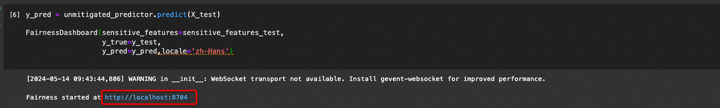
[公平性ダッシュボード] ページで、[開始] をクリックします。機密性の高い特徴量、パフォーマンスメトリック、公平性メトリックを構成して、グループ間で予測がどのように異なるかを分析します。
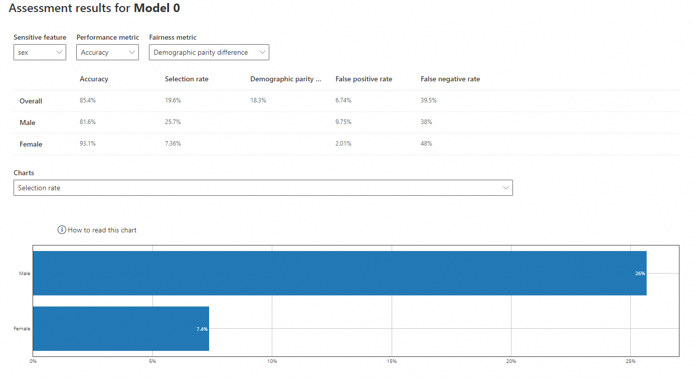
機密性の高い特徴量: sex
-
機密性の高い特徴量: sex
-
パフォーマンスメトリック: 精度
-
公平性メトリック: デモグラフィックパリティ差
-
精度: 正しい予測の割合。男性 (81.6%) に対するモデルの精度は女性 (93.1%) よりも低いですが、どちらも全体の精度 (85.4%) に近いです。
-
選択率: ポジティブな結果 (収入 >50K) を予測する確率。男性 (25.7%) の率は女性 (7.36%) よりも高く、女性の率は全体の率 (19.6%) よりもはるかに低いです。
-
デモグラフィックパリティ差: グループ間のポジティブな予測率の差。0 に近い値ほどバイアスが少ないことを示します。全体の差は 18.3% です。
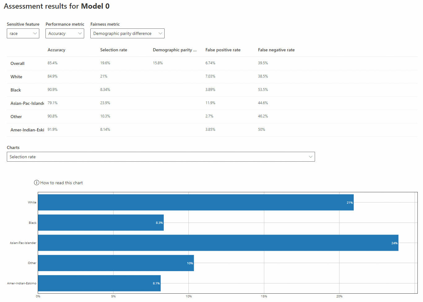
機密性の高い特徴量: race
-
機密性の高い特徴量: race
-
パフォーマンスメトリック: 精度
-
公平性メトリック: デモグラフィックパリティ差
-
精度: 'White' (84.9%) と 'Asian-Pac-Islander' (79.1%) に対するモデルの精度は、'Black' (90.9%)、'Other' (90.8%)、'Amer-Indian-Eskimo' (91.9%) よりも低いです。すべての値は全体の精度 (85.4%) に近いです。
-
選択率: 'White' (21%) と 'Asian-Pac-Islander' (23.9%) の率は、'Black' (8.34%)、'Other' (10.3%)、'Amer-Indian-Eskimo' (8.14%) よりも高いです。後者の 3 つは全体の率 (19.6%) よりもはるかに低いです。
-
デモグラフィックパリティ差: 全体の差は 15.8% です。