SPL instructions

0.0.201

The time-series Simple Log Service Processing Language (SPL) instructions are used to transform tabular data into time series data.

Instruction	Description

Instruction	Description
make-series	Builds tabular data into time series data.
render	Renders SPL query results as charts for visualization.

make-series

Constructs series structure from tabular data.

Syntax

| make-series  <output> = <field-col> [default = <default-value>]
             [, ...]
             on <time-col>
             [from <time-begin> to <time-end>
              step <step-value>]
             [by <tag-col>,...]

Instruction blocks

Instruction block	Required	Description

Instruction block	Required	Description
<output> = <field-col> , ...	Yes	Field columns to be converted to series, multiple columns can be selected.
on <time-col>	Yes	Field column with time meaning.
[default = <default-value>] & [from <time-begin> to <time-end> step <step-value>]	No	Fill missing values based on the time column. Includes time range to extract, fill step size, and fill strategy.
[by <tag-col>,...]	No	Aggregate by specified tag columns.

Parameter description

Parameter	Type	Description

Parameter	Type	Description
output	Field	Output field after aggregation.
field-col	Field	Input field column.
default-value	String	Missing value filling method. Valid values: null: Fill missing data points with null. nan: Fill missing floating-point numbers with nan. 0: Fill missing data points with 0. last: Use the last observed value to fill missing data points. Also known as forward filling. Suitable when you expect missing data to logically maintain the last known state before a new observation appears. Typically used in scenarios where values are considered unchanged until updated. next: Use the next observed value to fill missing data points. Also known as backward filling. Suitable when data might be considered to exist in some future state before being explicitly observed. Can be used when historical values are considered the same as the next observed value. avg: Use the average of the previous time point and the next time point to fill missing data points.
time-col	Field	Input time column.
time-begin	String or Field	Expected time column range, starting point. Valid values: Specific field name. A field of type bigint, where the value is the starting point in nanoseconds. min: Use the minimum value of each time series as the starting point. sls_begin_time: Use the query start time as the starting point for each time series.
time-end	String or Field	Expected time column range, ending point. Valid values: Specific field name. A field of type bigint, where the value is the ending point in nanoseconds. min: Use the maximum value of each time series as the ending point. sls_begin_time: Use the query end time as the ending point for each time series.
step-value	String	Missing value fill step size. Valid units: s (seconds), m (minutes), h (hours), d (days), w (weeks).
tag-col	Field	Aggregate by this field value.

Example

Construct a timeline from raw data time points and fill missing points.

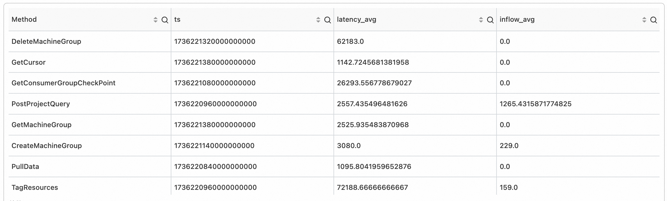
Raw data

For different methods, align timestamps by 60s and calculate aggregated metrics within the 60s time window to obtain time points.

SPL statement

* | extend ts = second_to_nano(__time__ - __time__ % 60)
  | stats latency_avg = avg(cast(latency as double)), inflow_avg = avg(cast (inflow as double)) by ts, Method

Output

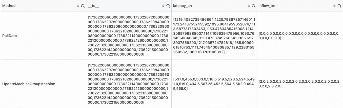
SPL statement

* | extend ts = second_to_nano(__time__ - __time__ % 60)
  | stats latency_avg = max(cast(latency as double)), inflow_avg = min(cast (inflow as double)) by ts, Method
  | make-series   latency_avg default = 'last',
                inflow_avg default = 'last'
                on ts
                from 'min' to 'max'
                step '1m'
                by Method

Output

render

Renders SPL query results as charts for visualization.

The render instruction must be the last operator in an SPL query.
The render instruction does not modify data. It only adds visualization parameters to the extended properties of the query results.

Syntax

render visualization [with ( propertyName = propertyValue [, ...])]

Instruction blocks

Instruction block	Required	Description

Instruction block	Required	Description
visualization	Yes	Indicates the type of visualization chart to use.
propertyName = propertyValue	No	A separated list of key-value property pairs. See the supported properties below.

Parameter description

Visualization

Visualization	Description

Visualization	Description
linechart	Line chart

Properties

PropertyName/PropertyValue key-value pairs indicate additional information to use when rendering charts. All properties are optional. Supported properties:

Parameter configuration for rendering time series forecasting charts

PropertyName	PropertyValue

PropertyName	PropertyValue
xcolumn	Column name in the query result to be used as the x-axis.
ycolumns	List of column names in the query result to be used as the y-axis, separated by commas.

For example:

... ...
| render linechart with (xcolumn=time_series,
                         ycolumns=metric_series, forecast_metric_series)

Parameter configuration for rendering anomaly detection charts

PropertyName	PropertyValue

PropertyName	PropertyValue
xcolumn	Column name in the query result to be used as the x-axis.
ycolumns	List of column names in the query result to be used as the y-axis, separated by commas.
anomalyscore	Display anomaly scores for anomaly points on the chart. Only applies to linechart.
anomalytype	Display anomaly types for anomaly points on the chart. Only applies to linechart.

For example:

... ...
| render linechart with (xcolumn=ts,
                         ycolumns=mem_arr, cpu_arr,
                         anomalyscore = anomalies_score_series,
                         anomalytype = anomalies_type_series)

Example

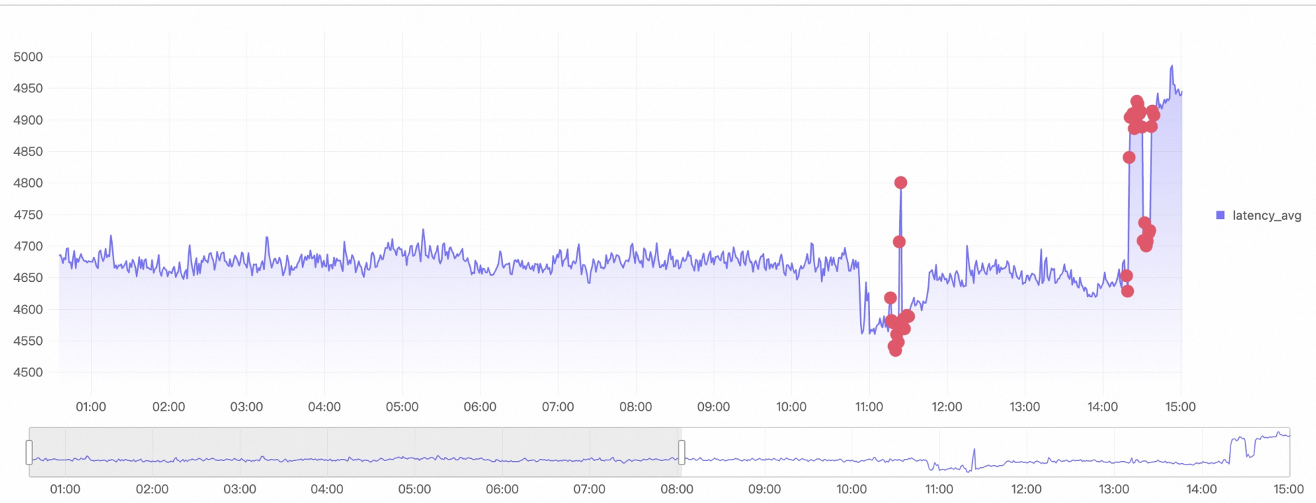
After anomaly detection on all timelines, retain the anomaly score values from the last 5 minutes and render an anomaly detection chart.

SPL statement

* 
| extend ts= (__time__- __time__%60)*1000000000
| where Method='PostLogStoreLogs'
| stats latency_avg=avg(cast( Latency as bigint)) by ts, Method
| make-series   latency_avg = latency_avg default = 'null'
                on ts
                from 'min' to 'max'
                step '1m'
                by Method
| extend ret = series_decompose_anomalies(latency_avg)
| extend anomalies_score_series = ret.anomalies_score_series, anomalies_type_series = ret.anomalies_type_series, error_msg = ret.error_msg
| render linechart with (xcolumn=__ts__,
                         ycolumns=latency_avg,
                         anomalyscore = anomalies_score_series,
                         anomalytype = anomalies_type_series)

Output

Feedback

Previous: Time-series SPLNext: Spl function

On this page （1）

SPL instructions

make-series

Syntax

Instruction blocks

Parameter description

Example

render

Syntax

Instruction blocks

Parameter description

Example

Chat now with Alibaba Cloud Customer Service to assist you in finding the right products and services to meet your needs.

SPL instructions