Tair (Redis® OSS-Compatible):TairVector performance whitepaper

TairVector supports the approximate nearest neighbor (ANN) search algorithm. You can use TairVector for semantic retrieval of unstructured data and personalized recommendations. For more information, see Vector.

Test description

Database test environment

Client test environment

• An Elastic Compute Service (ECS) instance that is deployed in the same virtual private cloud (VPC) as the Tair (Redis OSS-compatible) instance is created and is connected to the Tair (Redis OSS-compatible) instance over the VPC.

• The Linux operating system is used.

• Python 3.7 or later is installed.

Test data

The Sift-128-euclidean, Gist-960-euclidean, Glove-200-angular, and Deep-image-96-angular datasets are used to test the Hierarchical Navigable Small World (HNSW) indexing algorithm. The Random-s-100-euclidean and Mnist-784-euclidean datasets are used to test the Flat Search indexing algorithm.

Test tools and methods

1. Install tair-py and hiredis on the test server.

   Run the following command to install hiredis:

   pip install tair hiredis

2. Download and decompress Ann-benchmarks.

   Run the following command to decompress Ann-benchmarks:

   tar -zxvf ann-benchmarks.tar.gz

3. Configure the endpoint, port number, username, and password of the Tair instance in the algos.yaml file.

   Open the algos.yaml file, search for tairvector to find the relevant configuration items, and then configure the following parameters of base-args:

   • url: the endpoint, username, and password of the Tair instance. Format: redis://user:password@host:port.

   • parallelism: the number of concurrent threads. Default value: 4. We recommend that you use the default value.

   Example:

   {"url": "redis://testaccount:Rp829dlwa@r-bp18uownec8it5****.redis.rds.aliyuncs.com:6379", "parallelism": 4}

4. Run the run.py script to start the test.

   Important

   After you run the run.py script, the entire test is started to create an index, write data to the index, and then query and record the results. Do not repeatedly run the script on a single dataset.

   Example:

   # Run a multi-threaded test by using the Sift-128-euclidean dataset and HNSW indexing algorithm. 
   python run.py --local --runs 3 --algorithm tairvector-hnsw --dataset sift-128-euclidean --batch
   # Run a multi-threaded test by using the Mnist-784-euclidean dataset and Flat Search indexing algorithm. 
   python run.py --local --runs 3 --algorithm tairvector-flat --dataset mnist-784-euclidean --batch

   You can also use the built-in web frontend to execute the test. Example:

   # Install the Streamlit dependency in advance. 
   pip3 install streamlit
   # Start the web frontend. Then, you can enter http://localhost:8501 in your browser. 
   streamlit run webrunner.py

5. Run the data_export.py script and export the results.

   Example:

   # Multiple threads.
   python data_export.py --output out.csv --batch

Test results

We recommend that you pay more attention to the test results of write performance, k-nearest neighbor (kNN) query performance, and memory efficiency.

• Write performance: The write performance of TairVector increases in proportion to the write throughput.

• kNN query performance: The number of queries per second (QPS) reflects the system performance, and the recall rate reflects the accuracy of the results. Typically, the higher the recall rate, the lower the QPS. QPS comparison holds significance only if the recall rate is the same. In this context, the test results are presented with the "QPS v.s. Recall" curve. For FLAT indexes, only QPS is presented because the recall rate is always 1.

• Memory efficiency: The lower the memory usage of vector indexes, the better the performance of TairVector.

In this example, the performance of TairVector is tested with the float32 and float16 data types. The default data type is float32. The performance of the HNSW indexing algorithm is tested with the AUTO_GC feature enabled.

HNSW indexes

Write performance

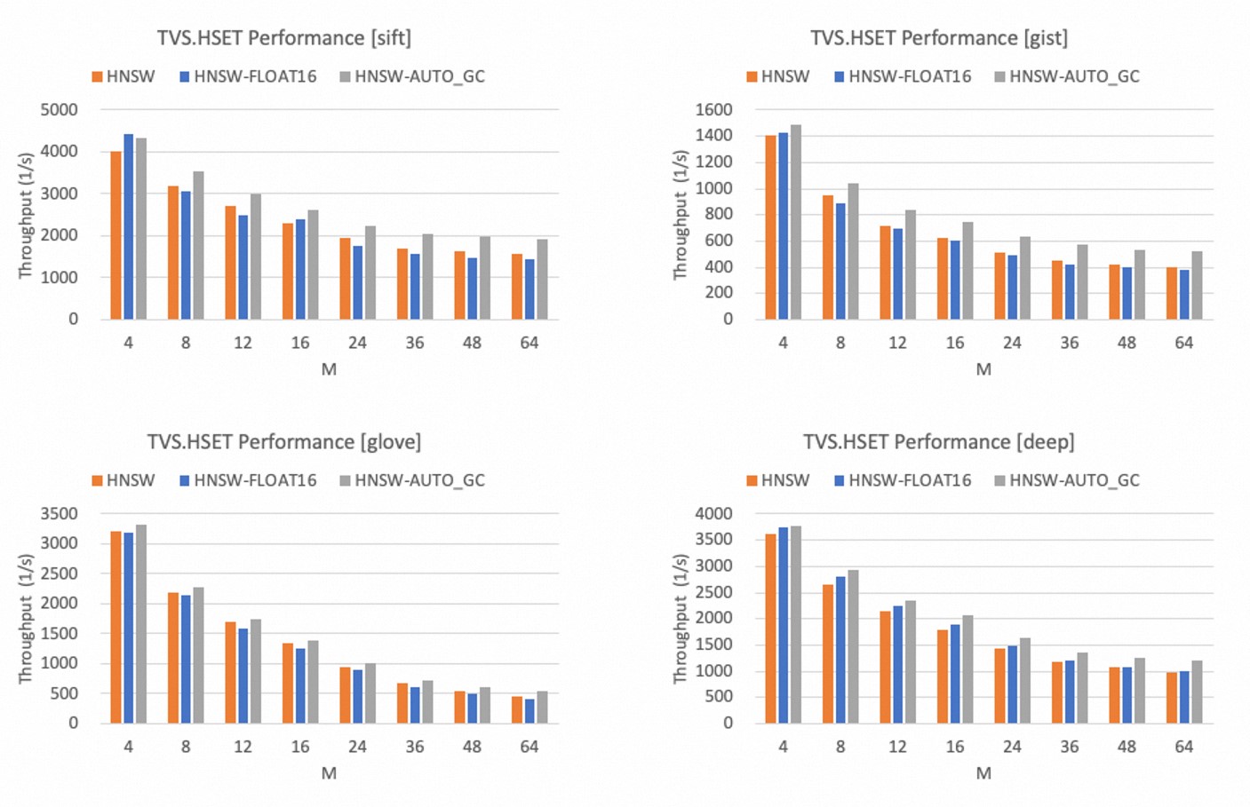
The following figures show the write performance of the HNSW indexing algorithm at different values of the M parameter when ef_construct is set to 500. The M parameter specifies the maximum number of outgoing neighbors on each layer in a graph index structure.

• The write performance of the HNSW indexing algorithm decreases in inverse proportion to the value of the M parameter.

• Compared with the float32 data type, the write performance of the HNSW indexing algorithm slightly decreases in most cases when the float16 data type is used.

• After the AUTO_GC feature is enabled, the write performance of the HNSW indexing algorithm increases by up to 30%.

kNN query performance

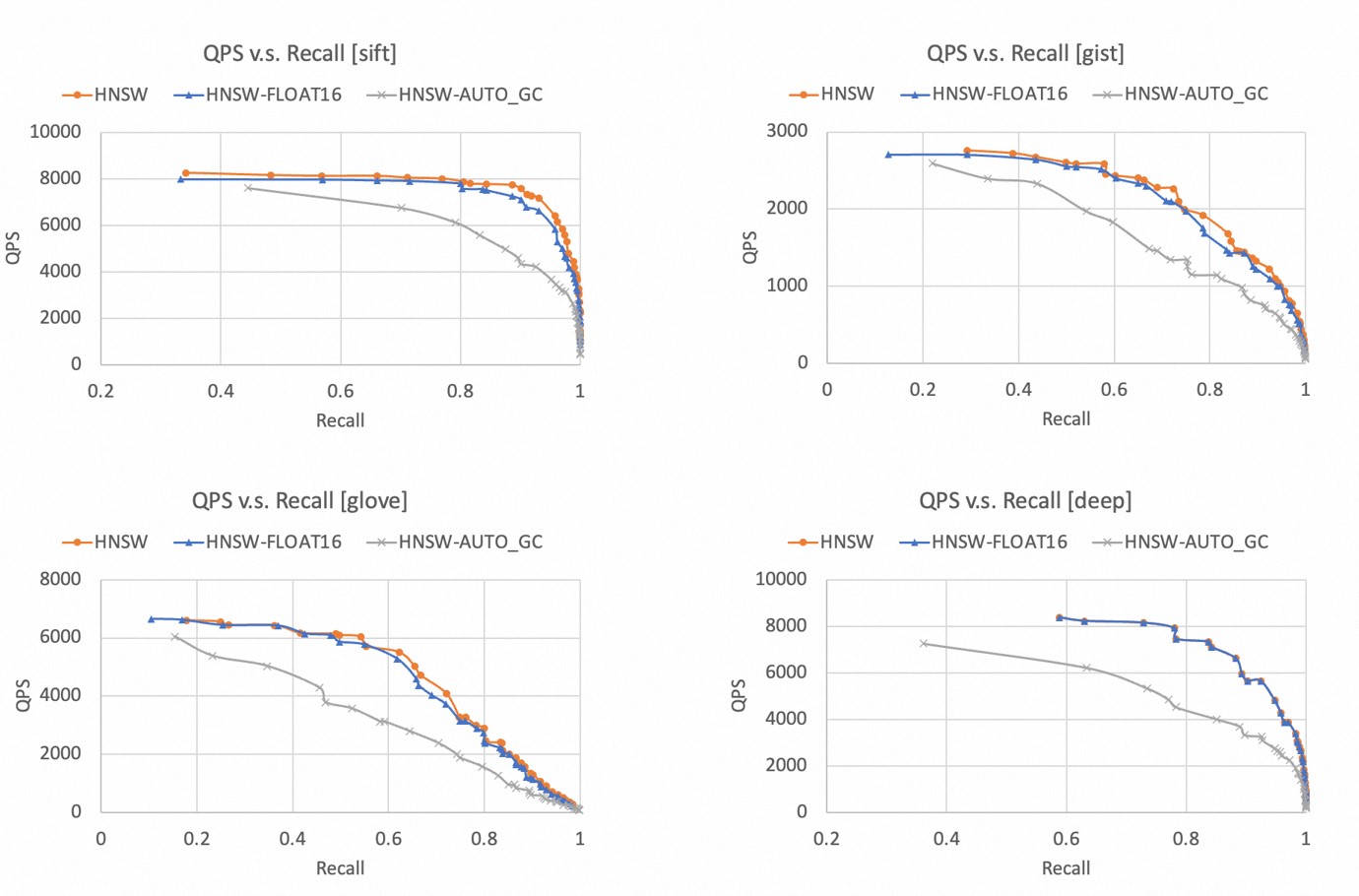
The higher the recall rate and QPS, the better the kNN query performance. Therefore, the closer the curve is to the upper-right corner, the better the performance of the HNSW indexing algorithm.

The following figures show the "QPS v.s. Recall" curves when HNSW indexes are used with different datasets.

• For all four datasets, HNSW indexes can achieve a recall rate of more than 99%.

• Compared with the float32 data type, the performance of the HNSW indexing algorithm slightly decreases when the float16 data type is used. The performance of these two data types is extremely close.

• After the AUTO_GC feature is enabled, the kNN query performance significantly decreases. Therefore, we recommend that you enable the AUTO_GC feature only when you want to delete a large amount of data.

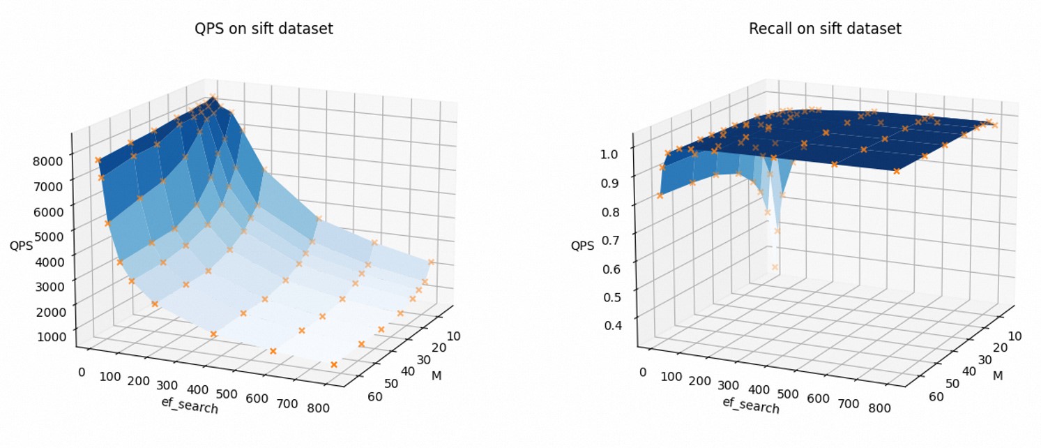
To visually present how parameter settings affect the kNN query performance, the following figures show how the QPS and recall rate change with the values of M and ef_search. In this example, the Sift-128-euclidean dataset and the float32 data type are used, and the AUTO_GC feature is disabled.

As the values of M and ef_search increase, the QPS decreases and the recall rate increases.

Memory efficiency

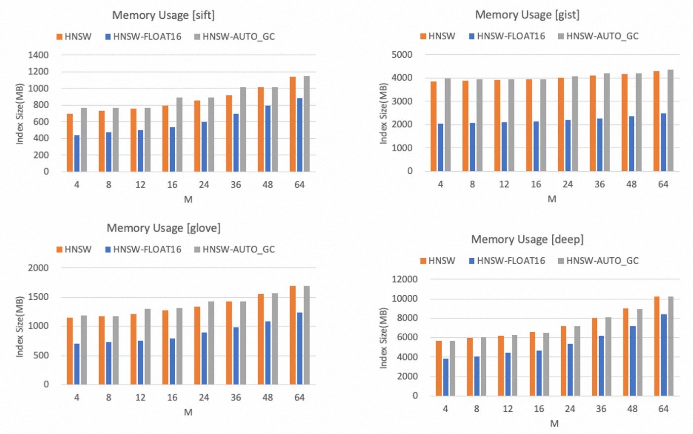
The memory usage of HNSW indexes increases only in proportion to the value of the M parameter.

The following figures show the memory usage of HNSW indexes between different datasets.

• Compared with the float32 data type, the float16 data type can significantly reduce the memory usage by more than 40%.

• After the AUTO_GC feature is enabled, the memory usage slightly increases.

  Note

  You can determine an appropriate value for the M parameter based on the dimension of vectors and your memory capacity budget. If you can accept a certain loss of precision, we recommend that you use the float16 data type to save memory space.

FLAT indexes

Write performance

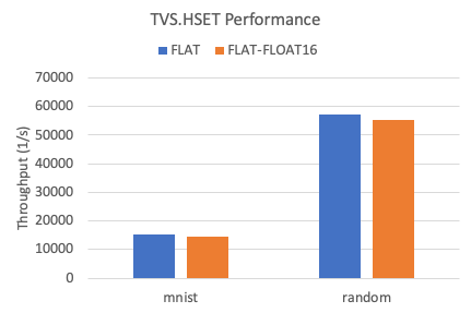
The following figure shows the write throughput of FLAT indexes between two datasets.

Compared with the float32 data type, the write performance of FLAT indexes decreases by approximately 5% when the float16 data type is used.

kNN query performance

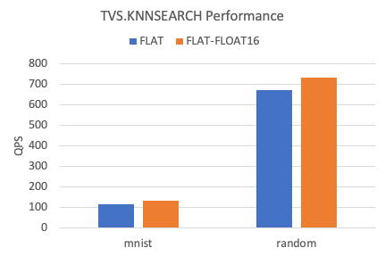
The following figure shows the kNN QPS of FLAT indexes between two datasets.

Compared with the float32 data type, the kNN query performance of FLAT indexes increases by approximately 10% when the float16 data type is used.

Memory efficiency

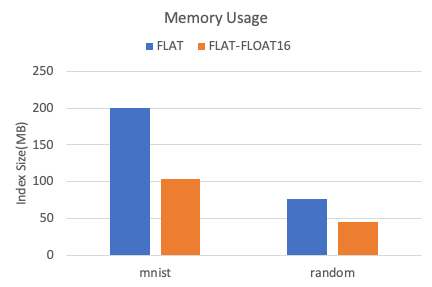
The following figure shows the memory usage of FLAT indexes between two datasets.

Compared with the float32 data type, the float16 data type can reduce the memory usage by more than 40%.