Double Eleven Technology Series: Logistics and Dynamic Path Planning

The Alibaba Cloud 2021 Double 11 Cloud Services Sale is live now! For a limited time only you can turbocharge your cloud journey with core Alibaba Cloud products available from just $1, while you can win up to $1,111 in cash plus $1,111 in Alibaba Cloud credits in the Number Guessing Contest.

Every year, the turnover for Alibaba's annual Double Eleven (Singles' Day) online shopping festival hits a record high, which poses a huge challenge to IT and logistics systems.

Thanks to the record-breaking annual shopping festival, warehouses in China are fully stocked with parcels every year. Given the astronomical number of transactions involved during this festival, how does the logistics industry keep up with the demands to ensure timely delivery of products?

Using Database Technologies to Optimize Logistics

The short answer to this question is by using database technologies such as Alibaba Cloud ApsaraDB for RDS PostgreSQL. Obviously, there is a lot more to that. That is why today, I want to share with you some of my knowledge and experience in applying database technologies to logistics. I will focus on PostgreSQL, Greenplum, and PostGIS.

The logistics industry is catalyzed by e-commerce. For the logistics industry, the scheduling algorithm for distributing and collecting parcels is the key to the efficient parcel distribution and collection as well as cost-effective operation of logistics companies. A good algorithm can boost efficiency and lower costs, and mobilize social resources to encourage nationwide participation, which is basically the entire business model of Didi taxi.

Taking the logistics industry as an example, I will analyze how PostgreSQL and Greenplum are applied in the logistics industry for geographical location information processing, optimal path calculation, and machine learning.

Element Analysis

At first glance, you may think that all a logistics enterprise do is simply sending and delivering parcels. But in fact, deciding on the right path is the key to enabling an optimal delivery system.

Let's first look at a simple logistic process as an example. The logistics process involves a number of elements in relation to the location.

Sender
Consignee: sends parcels to logistics sites instead of warehouses. Therefore, the routes from sites to warehouses should also be scheduled, which is not discussed herein.

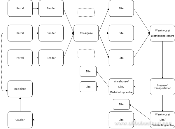
The scheduling method is similar to distribution:

Freight
Warehouse
Means of transportation
Deliverer
Recipient

If the time attribute is introduced, there is more room for imagination, as full participation can be envisaged like Didi Taxi does.

We will start with some simple elements that focus only on the location.

1. Sending a Parcel

Senders often need to make an appointment with the consignee for parcel sending. In addition, a sender can directly carry a parcel to a logistics site, so few algorithms are involved.

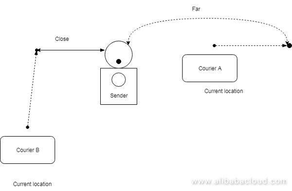
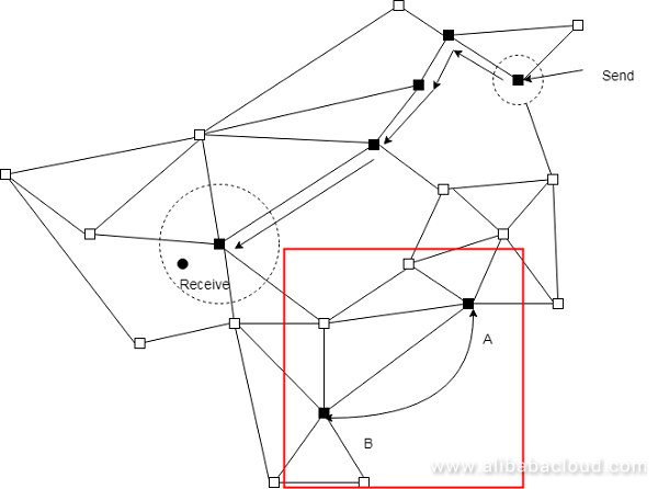
The k-NearestNeighbor (KNN) algorithm can solve the problem of mixing parcel delivery and collection together. Combined with delivery path scheduling, the optimal consignee can be selected.

For example, considering the current location of the sender and the next location of the courier, the cost will be the lowest if courier B is the one to collect the parcel according to the KNN algorithm.

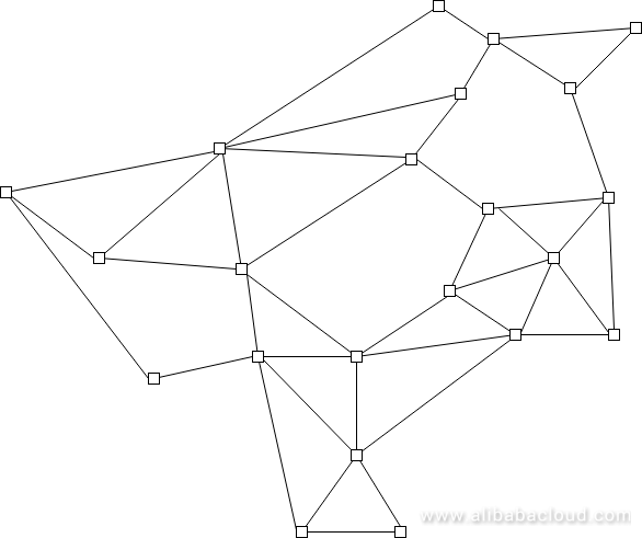
2. Scheduling of Parcel Transfers between Warehouses

Assume that the dots shown in the figure above are the locations of warehouses. If there is a path between two warehouses, the two warehouses are connected by lines. One warehouse covers a geometric area.

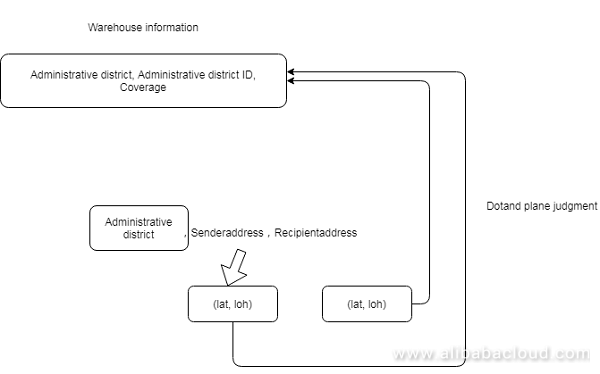
Based on locations of the sender and receiver as well as the area served by the warehouse, the dots and planes are combined to pinpoint the warehouses for the sender and receiver.

A parcel is seen as a dot and a warehouse is seen as a plane. When the sender sends a parcel, the sending and receiving information filled by the sender is translated into two longitudes and latitudes, based on which, coupled with the logistics company's warehouse map, the corresponding dots and planes are determined and matched. Hence, the start and end warehouses are determined for the parcel.

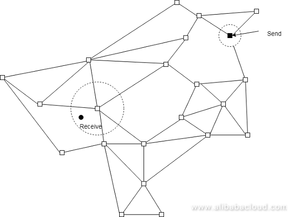
Dot and plane judgment

With a source and target, the optimal path for each parcel can be figured out by the optimal path algorithms from pgRouting.

A demo is provided later to explain how to use pgRouting to calculate the optimal path.

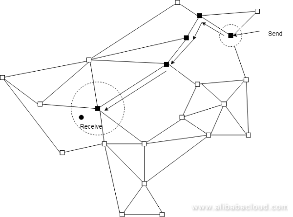
The freight car shipping parcels between warehouses can hit the road once the car is fully loaded, or in batches (considering time limitation). Instead of carrying the whole freight from the start point to the end point, a freight car is responsible for the whole trip between two nodes.

If a freight car is only responsible for path A-B, it ships parcels between node A and node B.

3. Scheduling of Parcel Transfers from the Destination Warehouse to a Logistics Site

After parcels arrive at the target warehouse, they will be sorted and sent to sites for delivery.

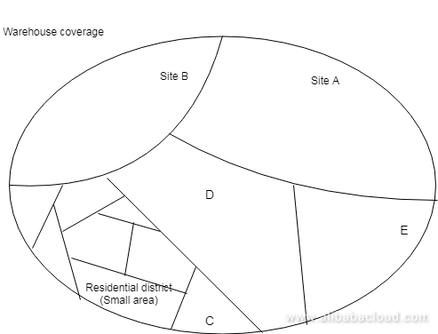
This is also a process of determining dots and planes. The plane refers to the area covered by a logistics site, while a parcel is seen as a dot. Based on dot and plane judgment, the optimal site is selected.

The principle for parcel transfer between warehouses also can be leveraged to calculate the optimal path to ship a parcel from a warehouse to a site. At the same time, a freight car is only responsible for shipping parcels between two sites.

4. Delivery

Delivery is what should be done in the last mile of sending a parcel to a receiver. To improve delivery scheduling, parcels should be aggregated based on their locations.

The principle for parcel transfer between warehouses can be applied again, which means the dots and planes should be determined again. However, the targets should be accurate to residential districts or smaller areas.

In addition to the destination (aggregated) of a parcel, the size and weight as well as the shipping capability (volume and weight) of a courier should be considered.

As shown in the figure below, all parcels at one logistics site need to be delivered to the following dots (aggregated). In addition, the total volume of parcels for each dot is shown in numbers.

Unlike the path planning mentioned above, this planning process focuses on multiple dots.

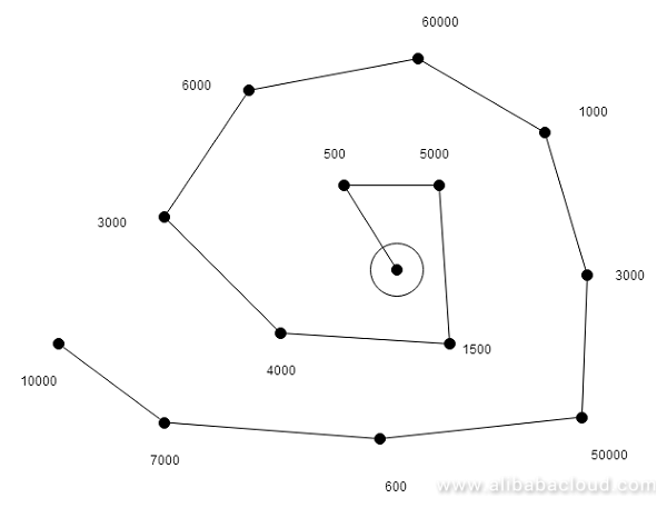
The purpose of calculating the optimal path for multiple destinations is to ensure that adjacent destinations are continuous and that a courier delivers parcels to adjacent destinations after parcels are sorted by sites.

For example, the logistics site is in the center, while other dots represent the destinations. The number around each destination refers to the parcel volume that one courier can carry each time. The dotted line refers to the parcels that one courier collects for one delivery.

This method ensures the continuity of parcels in each delivery.

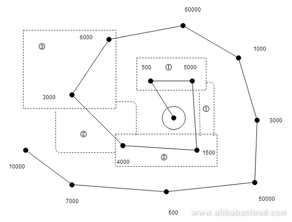
A demo is provided later to explain the optimal path planning for multiple destinations.

Location-Coordinate Conversion

This article does not discuss the conversion from locations into coordinates, while many navigation companies provide this capability.

A logistics company can use the couriers' hand-held GPS devices to obtain accurate coordinates. For example, a courier scans the parcel code while collecting the parcel to report the location information.

After some basic data are obtained, through text analysis and machine learning, the locations can also be converted into coordinates.

If there are enormous basic data, the Greenplum data warehouse based on PostgreSQL can be used for text analysis and machine learning (MADlib and R programming language supported).

Greenplum supports text analysis, geographical location information processing, MADlib machine learning library, custom function of R programming language, Python function, and parallel distributed computing. The most important thing is Greenplum is an open source data warehouse, which is the best choice for users who need to analyze texts and geographical locations.

Optimal Path Calculation

The data transfer between warehouses is used an example here.

The PostGIS and pgRouting of PostgreSQL are used.

https://workshop.pgrouting.org/2.5/en/chapters/topology.html

Basic data requirement, which refers to the data about line segments and kilometers of the activated transportation path between two warehouses.

Road link ID (gid): unique road ID

Road class (class_id)

Road link length (length): road length, in kilometers

Road name (name): road name

Road geometry (the_geom): road segment (segment among multiple points or between two points)

If the table name is ways, the information about line segments between warehouses is stored in the table.

               Table "public.ways"
  Column  |           Type            | Modifiers
----------+---------------------------+-----------
 gid      | bigint                    |
 class_id | integer                   | not null
 length   | double precision          |
 name     | character(200)            |
 osm_id   | bigint                    |
 the_geom | geometry(LineString,4326) |
Indexes:
    "ways_gid_idx" UNIQUE, btree (gid)
    "geom_idx" gist (the_geom)

1. Generate Topology

A valid topology should be generated before an optimal path is generated.

Before a topology is generated, two fields should be added to store the start and end code of a line segment.

-- Add "source" and "target" column
ALTER TABLE ways ADD COLUMN "source" integer;
ALTER TABLE ways ADD COLUMN "target" integer;

It should be noted that calling pgr_createTopology to generate a topology is the process of generating the first code for a line segment.

pgr_createTopology(
'<table>', which refers to the table for which a topology should be generated.
float tolerance, which refers to the allowed deviation when the end of a line segment cannot be completely fit. Generally, the unit for float tolerance is degree or kilometer.
'<geometry column>', which is the name of a line segment.
'<gid>')  --  gid

For example, there are three line segments: A, B, and C. Among them, the two ends of B cannot be fit with the ends of A and C. The deviations are 1 m and 10 m respectively, so the float tolerance should be set.

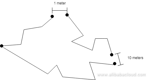
Generating a line segment is actually to set the source ID and target ID. After the setting, the result may be shown as follows.

Example:

-- Run topology function
SELECT pgr_createTopology('ways', 0.00001, 'the_geom', 'gid');

2. Generate an Optimal Path

pgRouting supports many optimal path algorithms, as described in the official documentation http://docs.pgrouting.org/2.2/en/doc/index.html

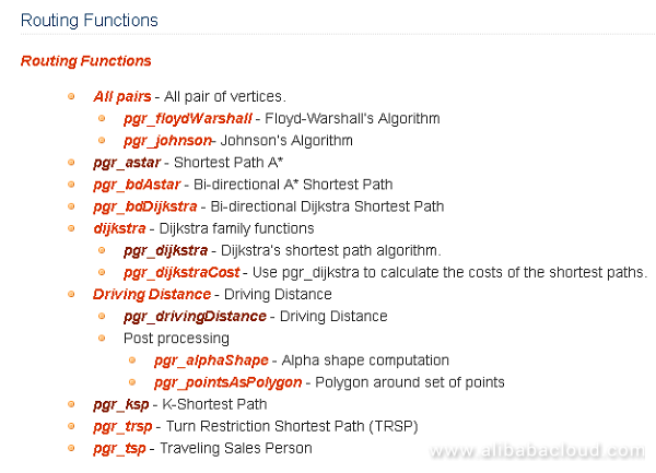
Taking Shortest Path A* and Shortest Path Dijkstra as examples, we will discuss how to generate an optimal path. https://workshop.pgrouting.org/2.5/en/chapters/shortest_path.html

What is the returning cost if there is a two-way line segment between two warehouses? If we should focus more on traffic jam for returning, in addition to cost incurred by path length, the cost incurred by traffic jam should also be considered.

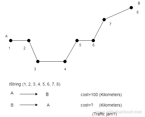
The calculation result using the returning cost by kilometers show that returning is supported in this line segment.

ALTER TABLE ways ADD COLUMN reverse_cost double precision;
UPDATE ways SET reverse_cost = length;

2.1 Example of Shortest Path Dijkstra algorithm

Call

pgr_costResult[] pgr_dijkstra(
text sql, which is used to calculate the data source of an optimal path and represented in SQL. For example,
--SELECT id (gid), source (start point ID of a line segment), target (end point ID of a line segment), cost (the cost from the start point to the end point) [,reverse_cost (cost from the end point to the start point)] FROM edge_table
integer source, which is the start point of a planned path.
integer target, which is the end point of a planned path.
boolean directed,   --  if the graph is directed
boolean has_rcost  -- if true, the reverse_cost column of the SQL generated set of rows will be used for the cost of the traversal of the edge in the opposite direction.
);

Rows that make up a path.

a set of pgr-costResult (seq (sequence, id1 (start point ID), id2 (target ID; -1 indicates the end point), cost (the cost spent on the line segment)) rows, that make up a path.

Example

The optimal path from 30 to 60.

SELECT seq, id1 AS node, id2 AS edge, cost FROM pgr_dijkstra('
                SELECT gid AS id,
                         source::integer,
                         target::integer,
                         length::double precision AS cost
                        FROM ways',
                30, 60, false, false);

 seq | node | edge |        cost
-----+------+------+---------------------
   0 |   30 |   53 |  0.0591267653820616
   1 |   44 |   52 |  0.0665408320949312
   2 |   14 |   15 |  0.0809556879332114
   ...
   6 |   10 | 6869 |  0.0164274192597773
   7 |   59 |   72 |  0.0109385169537801
   8 |   60 |   -1 |                   0
(9 rows)

2.2 Example of Shortest Path A* algorithm

The algorithm is similar to the Shortest Path Dijkstra algorithm, but the coordinates of the start and end points of a line segment should be used for SQL. Other parameters are the same as those used for pgr_dijkstra.

ALTER TABLE ways ADD COLUMN x1 double precision;
ALTER TABLE ways ADD COLUMN y1 double precision;
ALTER TABLE ways ADD COLUMN x2 double precision;
ALTER TABLE ways ADD COLUMN y2 double precision;

UPDATE ways SET x1 = ST_x(ST_PointN(the_geom, 1)), which is the coordinate x of the start point of a line segment.
UPDATE ways SET y1 = ST_y(ST_PointN(the_geom, 1)), which is the coordinate y of the start point of a line segment.

UPDATE ways SET x2 = ST_x(ST_PointN(the_geom, ST_NumPoints(the_geom))), which is the coordinate x of the end point of a line segment.
UPDATE ways SET y2 = ST_y(ST_PointN(the_geom, ST_NumPoints(the_geom))), which is the coordinate y of the end point of a line segment.

Call

pgr_costResult[] pgr_astar(
sql text,     --SELECT id, source, target, cost, x1, y1, x2, y2 [,reverse_cost] FROM edge_table, which contains the coordinates of the start and end points. This algorithm works a little bit faster than Shortest Path A*.
source integer,   
target integer, 
directed boolean, 
has_rcost boolean  
);

The return result is the same as that of pgr_dijkstra.

a set of pgr_costResult (seq, id1, id2, cost) rows, that make up a path.

Example

SELECT seq, id1 AS node, id2 AS edge, cost FROM pgr_astar('
                SELECT gid AS id,
                         source::integer,
                         target::integer,
                         length::double precision AS cost,
                         x1, y1, x2, y2
                        FROM ways',
                30, 60, false, false);

Result

 seq | node | edge |        cost
-----+------+------+---------------------
   0 |   30 |   53 |  0.0591267653820616
   1 |   44 |   52 |  0.0665408320949312
   2 |   14 |   15 |  0.0809556879332114
   ...
   6 |   10 | 6869 |  0.0164274192597773
   7 |   59 |   72 |  0.0109385169537801
   8 |   60 |   -1 |                   0
(9 rows)

3. Generate Multiple Optimal Paths for Multiple Targets

We can choose midway points for navigation, which is common for planning multiple targets. For example, you want to stay a night in your mother-in-law's house in Jiangshan on your way from Hangzhou to Wanzai.

In this example, the algorithm used is Multiple Shortest Paths with kDijkstra. This algorithm is used similarly to kDijkstra except one parameter. The targets are expressed by arrays.

Generate the segment-based cost

pgr_costResult[] pgr_kdijkstraCost(text sql, integer source,
                 integer[] targets, boolean directed, boolean has_rcost);

Example

Starting from 10 and arriving at 60, 70, and 80.

SELECT seq, id1 AS source, id2 AS target, cost FROM pgr_kdijkstraCost('
                SELECT gid AS id,
                         source::integer,
                         target::integer,
                         length::double precision AS cost
                        FROM ways',
                10, array[60,70,80], false, false);

 seq | source | target |       cost
-----+--------+--------+------------------
   0 |     10 |     60 | 13.4770181770774
   1 |     10 |     70 | 16.9231630493294
   2 |     10 |     80 | 17.7035050077573
(3 rows)

Generate a path

pgr_costResult[] pgr_kdijkstraPath(text sql, integer source,
                 integer[] targets, boolean directed, boolean has_rcost);

Example

Starting from 10 and arriving at 60, 70, and 80.

SELECT seq, id1 AS path, id2 AS edge, cost FROM pgr_kdijkstraPath('
                SELECT gid AS id,
                         source::integer,
                         target::integer,
                         length::double precision AS cost
                        FROM ways',
                10, array[60,70,80], false, false);

         seq | path | edge |        cost
-----+------+------+---------------------
   0 |   60 | 3163 |   0.427103399132954
   1 |   60 | 2098 |   0.441091435851107
...
  40 |   60 |   56 |  0.0452819891352444
  41 |   70 | 3163 |   0.427103399132954
  42 |   70 | 2098 |   0.441091435851107
...
 147 |   80 |  226 |  0.0730263299529259
 148 |   80 |  227 |  0.0741906229622583
(149 rows)

Conclusion

Technologies mentioned in this article include

Dot and plane judgment: After determining the dot and plane, perform aggregate operations based on planes.
Path planning
Supported optimal algorithms: Many algorithms are supported.
UDF: PostgreSQL supports a variety of languages for custom functions, including Python, R, and C.
Machine learning: PostgreSQL and Greenplum support MADlib. For R users of Greenplum, Greenplum can be used to mine parallel data implicitly and a large amount of data.
Location-coordinate conversion
Clustering algorithm: If the information about a residential district is stored in the database as a dot instead of a plane, the K-Means clustering algorithm of PostgreSQL or Greenplum can be used to determine the dot and plane for delivery. The same purpose can be achieved by aggregating the parcel with the residential district.

Example:

    SELECT kmeans(ARRAY[x, y, z], 10) OVER (), * FROM samples;
    SELECT kmeans(ARRAY[x, y], 2, ARRAY[0.5, 0.5, 1.0, 1.0]) OVER (), * FROM samples;
    SELECT kmeans(ARRAY[x, y, z], 2, ARRAY[ARRAY[0.5, 0.5], ARRAY[1.0, 1.0]]) OVER (PARTITION BY group_key), * FROM samples;

The first parameter is an array that should be analyzed through clustering analysis. The second parameter is eventually divided into categories (when the result is output, the category starts from 0. If there are two categories, 0 and 1 are output).

The third parameter is a seed parameter, which can be a one- or two-dimensional array. If it is a one-dimensional array, the third parameter should be the element number of the first parameter times the value of the second element. (It can be considered that each category is assigned with one seed.)

The seed array that we should assign is the dot array consisting of residential districts or office buildings covered by a logistics site.

In terms of processing geographical location information, PostgreSQL has been a leader serving a massive user base. PostGIS and pgRouting are two plugins for processing geographical location information.

PostGIS and pgrouting can be obtained from Alibaba Cloud ApsaraDB for RDS PostgreSQL.

Have fun and you are welcome anytime to discuss your business requirements with Alibaba Cloud. We look forward to seeing you again.

Community

Double Eleven Technology Series: Logistics and Dynamic Path Planning

Using Database Technologies to Optimize Logistics

Element Analysis

1. Sending a Parcel

2. Scheduling of Parcel Transfers between Warehouses

3. Scheduling of Parcel Transfers from the Destination Warehouse to a Logistics Site

4. Delivery

Location-Coordinate Conversion

Optimal Path Calculation

1. Generate Topology

2. Generate an Optimal Path

3. Generate Multiple Optimal Paths for Multiple Targets

Conclusion

Read previous post:

Read next post:

digoal

You may also like

Comments

digoal

Related Products

Black Friday Cloud Services Sale

PolarDB for PostgreSQL

AnalyticDB for PostgreSQL