Alibaba Engineers Have Worked out Loads of Methods to Detect Anomalies

In this blog, we will explore detecting anomalies from multiple angles and see how Alibaba engineers have worked out several different methods to do just that.

By Li Weibin, Hu Yi, and Wang Hao.

The dark web and black markets are going larger and larger nowadays, and new methods for cheating the system are constantly popping up. These issues can make advertising less effective or even lead to sharp increases in app promotion costs. Therefore, as you can imagine, the precise identification of these issues, specifically these cheating methods, is an important expectation of any Internet company or advertiser.

In this blog, we will be exploring the issues of anomaly detection from multiple angles and see how Alibaba engineers have worked out several different methods for detecting anomalies. Some of the angles that the Alibaba engineers worked out are time series data, statistics, distance data, and the linear methods. In this blog, we will look into these angles as well as many, many others.

But, before we get to into it, let's first discuss some background information.

Outlier detection is a process of detecting objects whose behavior are significantly different from that of the expected objects. These detected objects are called outliers. Outlier detection is widely used in production and life, such as anti-fraud for credit cards, industrial damage detection, and advertisement anti-cheating.

An outlier is a data object that is distinctly different to other data objects. As shown in Figure 1 below, the points in the N1 and N2 regions are normal data sets. However, points in O1, O2 and O3 regions do not fit into the normal patterns that you'll find with N1 and N2, and so they are outliers.

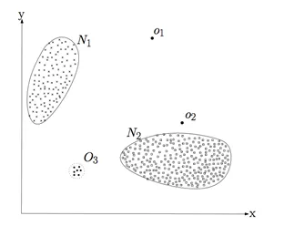
Figure 1. Example of outliers

One of the difficulties in anomaly detection is the lack of ground truth, which just simply means information that is not inferred. A common method to fix this is to use unsupervised methods to mine abnormal samples, and then use supervised models to fuse multiple features to mine more cheating.

Recently, multiple algorithms have been used to mine outliers. The following sections look into the principle and application scenarios of the anomaly detection algorithm from several different angles. Due to service specificity, of course, this article does not cover all feature details.

1. Time Series

1.1 Moving Average (MA)

Moving Average (MA) is a commonly used means for analyzing time series. It can filter high-frequency noise and detect outliers. Based on different computation methods, common MA algorithms include simple moving average, weighted moving average, and exponential moving average. Assume that the MA time window is T and a time series is provided:

1.1.1 Simple Moving Average (SMA)

It is easy to see from the above formula that the average of the historical value can be used as the predicted value of the current value. In the scenario where the sequence value fluctuates less with time, if the difference between the above moving average and the real value at that time exceeds a certain threshold, the value at that time is determined to be abnormal.

Applicable to:

Smooth the noise data, that is, replacing the current time value with the moving average to filter noise.
Predict future values.

1.1.2 Weighted Moving Average (WMA)

As the Simple Moving Average (SMA) gives the same weight to all data points in the window, it is not sensitive to more recent data, and the predicted value may be lagging. Following this line of thinking, it will naturally give a higher weight to more recent data when computing the moving average, while giving a lower weight to older data within the window, so as to capture the recent changes faster. Thus, the Weighted Moving Average (WMA) and the Exponential Moving Average (EMA) are obtained.

The WMA is more sensitive to recent changes than the SMA. The WMA has less lag than the SMA. However, the WMA still has a certain lag because the weight only decreases linearly.

1.1.3 Exponential Moving Average (EMA)

The Exponential Moving Average (EMA) is similar to the Weighted Moving Average (WMA), but the difference is that the weight of each value decreases exponentially instead of linearly. In addition, for the exponential decreases, no matter how old the data is, the coefficient of the data in this period will not decrease to 0, but only approach 0. Therefore, the EMA is actually an infinite series, that is, no matter how old the data is, it will play a certain role in computing the current EMA, but the weight of the data that is too far away from the current time is very low. In practical application, the EMA at time "t" can be obtained as follows:

indicates the degree of weight decrease. The value ranges from 0 to 1. The larger the value, the faster the observed values in the past decrease.

1.2 Year-on-Year Ratio and Month-over-Month Ratio

Figure 2. Year-on-Year ratio and Month-over-Month ratio

The Year-on-Year and Month-over-Month formulas are shown in Figure 2. They are suitable for use in scenarios with periodic data. For example, it can be used for monitoring the Year-on-Year and Month-over-Month ratio for daily active users (DAU) of the app, to detect whether the number of daily active users (DAU) is rising or falling during a given period of time. As a second example, it can also be used for monitoring the real-time Year-over-Year and Month-over-Month ratio for clicks and consumption of advertisements, to detect changes over time. When the above ratio exceeds a certain threshold (for information on the threshold, please see section 10), it is determined that an anomaly occurs.

1.3 Anomaly Detection of Time Series Metrics (STL + GESD)

STL is a single-dimension anomaly detection algorithm for time series metrics. The general idea is:

To decompose the metrics into STL time series first, to obtain the Seasonal, Trend, and Residual components, as shown in Figure 3.
To use the GESD (which stands for generalized extreme studentized deviate) algorithm to detect the anomaly of the Trend and Residual components.
To replace the mean and std statistics in the GESD algorithm with median and MAD (median absolute deviation), to improve the robustness against the outlier.
To output the anomaly score: abnorm_score = (value - median)/MAD, where the "value" is the current value, and "median" is the median of the sequence. A negative score indicates a decrease in anomalies, while a positive score indicates an increase in anomalies.

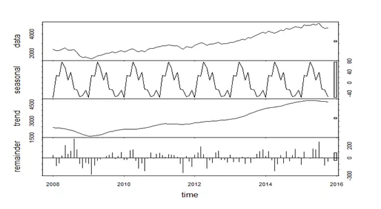
Figure 3. STL decomposition example

2. Statistics

2.1 Single Feature, Which Conform to Gaussian Distribution

If the variable x follows the Gaussian distribution , then its probability density function is:

We can use the existing sample data to predict the in the population. The computation method is as follows:

2.2 Multiple Unrelated Features, All of Which Conform to Gaussian Distribution

Assume that an n-dimensional dataset looks like this:

And each variable conforms to Gaussian distribution, then the average and variance of each dimension can be computed.

Specifically, for , the following can be computed:

If a new piece of data is provided, the probability can be computed as follows:

2.3 Multiple Related Features, Which Conform to Multivariate Gaussian Distribution

Assume that an n-dimensional dataset is , and each variable conforms to Gaussian distribution, then the covariance matrix of the n-dimensional average vector can be computed:

If a new piece of data is provided, the probability can be computed:

2.4 Mahalanobis Distance

For a multi-dimensional column vector dataset D, assuming that is an average vector, then for any object in the dataset D, the Mahalanobis distance from to is:

is the covariance matrix. The value can be sorted. If the value is too large, then the point can be considered as an outlier.

2.5 Boxplot

The boxplot algorithm does not require data to be subject to a specific distribution. For example, this method can be used even if the data distribution does not conform to Gaussian distribution. This method needs to compute the first quartile Q1 (25%) and the third quartile Q3 (75%). Let IQR = Q3-Q1, and then compute the outlier boundary points Q3 + λIQR and Q1- λIQR. Usually, λ takes a value of 1.5 (similar to in normal distribution). As shown in Figure 4 below:

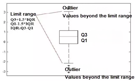
Figure 4. Schematic diagram of boxplot algorithm

3. Distance

3.1 Angle-Based Outlier Detection

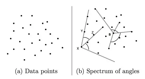
Figure 5. Point set and angle

As shown in Figure 5 above, three points X, Y, and Z, and two vectors exist now. If the change of angle is small for any different point, such as Y and Z, then point X is an outlier. The angle is easily obtained using the cosine-angle formula:

If D is a point set, then for any different point , the variance of all angles of point X is:

The above variance of the outlier is small. The time complexity of the algorithm is , which is suitable for scenarios with a small data volume N.

3.2 KNN-Based Outlier Detection

If D is a point set, then for any point , the sum of distances Dist(K,X) of its K nearest neighbors is computed. The greater the Dist(K,X), the more abnormal the point. The time complexity is , where N is the size of the data amount.

4. Linear Method (Matrix Decomposition and PCA Dimension Reduction)

The main idea of the matrix decomposition-based outlier detection method is to use Principal Component Analysis (PCA) to find outliers that violate the correlation between data. To locate these outliers, the PCA-based algorithm projects data from the original space to the principal component space, and then from the principal component space to the original space. For most data, if only the first principal component is used for projection and reconstruction, the error after reconstruction is small. However, for outliers, the error after reconstruction is relatively large. This is because the first principal component reflects the variance of normal points, and the last principal component reflects the variance of outliers.

Assume that X is a p-dimensional dataset with N samples, and its covariance matrix is . Then, the covariance matrix can be decomposed as

P is a -dimensional orthogonal matrix, , and each of its columns is an eigenvector. D is a -dimensional diagonal matrix, which contains eigenvalues . On a graph, an eigenvector can be regarded as a line in a 2-dimensional plane, or a plane in a higher dimensional space. The eigenvalues corresponding to the eigenvectors reflect the stretching degree of the batch of data in this direction. Generally, the eigenvalues in the eigenvalue matrix D are sorted from large to small, and each column of the eigenvector matrix P is adjusted accordingly.

The projection of dataset X on the principal component space can be written as Y = XP. Note that the projection can be performed only on some dimensions. The matrix after the principal component projection of top-j is:

is the first j column(s) of matrix p, that is, is a -dimensional matrix. is the first j column(s) of matrix Y and is a -dimensional matrix. In the same way, the data is projected from the principal component space to the original space. The reconstructed dataset is .

The data set restructured by using the principal component of top-j is a dimension matrix. The matrix is shown in Figure 6.

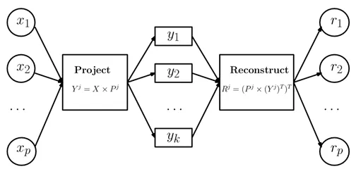
Figure 6. Matrix transformation diagram

The outlier of

is defined as:

where represents the ratio of the principal component of top-j to all the principal components. The eigenvalues are sorted in descending order. Therefore, is incremental, which means the larger the j value, the more the variances included in , because this is the summation from 1 to j. In this definition, the first principal component with the biggest deviant receives the smallest weight and the last principal component with the smallest deviant receives the biggest weight (1). Due to the characteristics of PCA, outliers have a relatively large variance on the last principal component, leading to a larger anomaly score.

5. Distribution

The policy is to compare the distribution of a feature of the benchmark traffic and that feature of the traffic to be detected.

5.1 Relative Entropy (KL Divergence)

The relative entropy (KL divergence) can measure the distance between two probability distributions. When two probability distributions are the same, their relative entropy is zero. If the difference between the two probability distributions increases, their relative entropy will increase accordingly. Therefore, the relative entropy can be used to compare the similarity of two probabilities. Given two probability distributions , the relative entropy is .

5.2 Chi-square Test

A chi-square test can be used to compare the difference between the expected result and the observed result by using the test statistics and obtain the probability of the observed result. In the test statistics, O represents the observed value and E the expected value. The test statistics provides a method to measure the difference between the expected result and the observed result. The final determination is based on the probability table according to the significance level that has been set.

6. Tree (Isolation Forest)

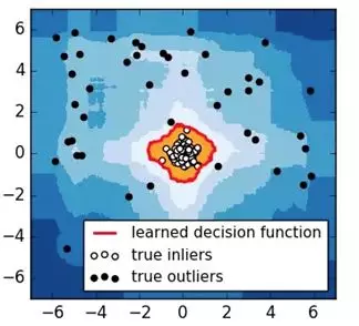
Figure 7. iForest detection result

Isolation Forest: Suppose that we use a random hyperplane to split the data space. Each split can generate two sub-spaces. Then we keep splitting individual sub-spaces by using a random hyperplane until each sub-space contains only one data point. Clusters with a high density need to be split many times before each sub-space contains only one data point. However, a sub-space where the data point density is low can quickly be further split into smaller sub-spaces with each containing only one data point. As shown in Figure 7, the black points are outliers, which are included in a sub-space after the space is split several times; the white points are normal points, which are converged in a cluster. The outlier boundary detected by the isolation forest is the red line in Figure 7. The isolation forest can correctly detect all the black outliers.

As shown in Figure 8, iForest is used to divide four data entries. The height of b and c is 3, the height of a is 2, and the height of d is 1. Because d is isolated first, it is most likely to be an outlier.

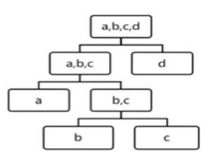
Figure 8. iForest isolation

7. Graph

7.1 Maximal Connected Subgraph

In the undirected graph G, vertex A is connected to vertex B if a path exists between them. Graph G contains several subgraphs, where each vertex is connected to every other vertex in the same subgraph but is separated from those in other subgraphs. These subgraphs of graph G are maximum connected subgraphs.

Figure 9 shows the connections between device IDs and mbr IDs. An edge between two nodes indicates that the corresponding member has logged on to a specific device. From Figure 9, we know that the same member has logged on to device_1, device_2, device_3, and device_4. This can be used to determine fraud in certain scenarios, usually for spotting coordinated fraud groups.

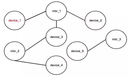
Figure 9. Maximal connected subgraph result

The premise of the maximal connected subgraph is that each edge must have confidence. Applicable scenario: Find all connections. When an edge with low confidence exists, dirty data needs to be removed. Otherwise the validity of the maximal connected subgraph would be reduced.

7.2 Label Propagation for Clustering

The label propagation algorithm for graph clustering is used to divide a graph into subgraphs based on the topology of the graph so that the links between the nodes in a subgraph are more than the links between the subgraphs. The basic idea of the label propagation algorithm is that the label of a node depends on the label information of its neighboring nodes. The impact level is decided by the node similarity. Labels are propagated, iterated and updated to reach a stable status. Two subgraphs are obtained for the nodes in Figure 10 after the labels are propagated for clustering, where nodes 1, node 2, node 3, and node 4 belong to the same subgraph and node 5, node 6, node 7, and node 8 belongs to the other subgraph.

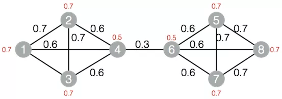
Figure 10. Graph structure of the label propagation algorithm for clustering

A small number of links are allowed between the subgraphs of the label propagation for clustering. Applicable scenario: High cohesion and low coupling between nodes. In Figure 10, a subgraph is obtained from the maximal connected subgraph, and two subgraphs are obtained from the label propagation algorithm for clustering.

8. Behavior Sequence (Markov Chain)

As shown in Figure 11, users have five behavior states on the search engine: page request (P), search (S), natural search result (W), add click (O), and page turning (N). State transition may happen between states. A chain composed of several behavior states can be considered a Markov chain.

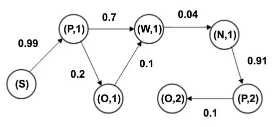
Figure 11. User behavior state chart

To obtain a state transition matrix, we can collect any two adjacent states in a normal behavior sequence and calculate the probability of each state transiting to any other state. For each user behavior sequence to be detected, we can easily find the probability of that sequence. The larger the probability, the more normal the user behaviors are.

9. Supervised Models

The preceding methods are relatively simple and easy to implement, because none of them involve supervision. However, because some of these methods only use a small number of features each time, we need to maintain lots of policies to intercept fraud in a comprehensive way. In addition, the effect of combining some of the aforementioned methods for multiple features depends on personal experience. Supervised models can automatically combine many features and provide a more powerful generalization ability.

9.1 Machine Learning Model GBDT

Sample: Use the fraud samples mined by using the preceding unsupervised methods as the training samples. If the number of the fraud samples is still small, use Synthetic Minority Over-sampling Technique (SMOTE) or Generative Adversarial Net (GAN) to generate more fraud samples. Then train a gradient boosting decision tree (GBDT) and use the transformation data to evaluate the model.

9.2 Deep Learning Model Wide & Deep

Wide & Deep extracts wide features and deep features respectively and then merge them for training. The model structure is shown in Figure 12. Wide refers to the LR of high-dimensional features and feature combinations. LR is efficient, scalable and strongly interpretable. The constant enhancement of feature combinations will facilitate memorization of the model judgement. However, the generalization ability of LR is weak.

Deep uses neural network to freely combine and map features and features strong generalization. Deep extracts more common characteristics of the sample features for judgement, but this may lead to excessive generalization.

The algorithm combines the two types of features to achieve a balance between memorization and generalization.

To further strengthen the generalization ability of the model, we can use the samples mined by using the unsupervised methods in the preceding sections as our training samples for training the Wide & Deep model to identify fraud.

Figure 12. Wide & Deep model

10. Other Problems

10.1 Common Threshold Selection Methods

All the preceding methods involve the computation of anomaly threshold. We can select a threshold by using the following methods and then use the transformation data to verify the rationality of the selected threshold.

Unsupervised methods: Use the quantile threshold and locate the inflection point of the distribution curve of historical data.
Supervised models: Check the accuracy curve and the recall curve of the validation sets.

10.2 Transform Non-Gaussian Distributions to Gaussian Distributions

Some features do not conform to the Gaussian distribution. We can use functions to transform them so that they become compliant with the Gaussian distribution and the aforementioned statistics methods can be used. A common transformation function is , where c is a non-negative constant. Another common transformation function is , where c is a fraction between 0 and 1.

References:

[1] Charu C, Aggarwal, et al. Outlier Analysis Second Edition, Springer. 2016
[2] Varun Chandola, Arindam Banerjee, et al. Anomaly Detection: A survey, ACM Computing Surveys. 2009
[3] Kalyan Veeramachaneni, Ignacio Arnaldo, et al. AI2: Training a big data machine to defend, In Proc. HPSC and IDS. 2016
[4] Liu, Fei Tony, Kai Ming Ting, and Zhi-Hua Zhou, et al. Isolationforest, ICDM. 2008
[5] Cheng H T, Koc L, Harmsen J, et al. Wide & Deep Learning for Recommender Systems, ACM Computing Surveys. 2016
[6] SMOTE: Synthetic Minority Over-sampling Technique, JAIR. 2002

5615908183575841 December 17, 2020 at 5:42 am

In Part 10.2, what is the "transformation function" ? It seems missing due to text format?

: weibin December 17, 2020 at 8:19 am

yeah ,thanks for reminding.A common transformation function is :y = log(x),y = x^2, y = log(x c),where c is a non-negative constant ; transformation function is y=x^c, where c is a fraction between 0 and 1.

0