A support vector machine (SVM) is a machine learning model that is developed based on the statistical learning theory. It minimizes risks and improves the generalization capability of learning machines. This way, empirical risks and confidence intervals are minimized. This topic describes how to configure the Linear SVM component and provides an example on how to use the component.
Background information
The Linear SVM component is not implemented by using kernel functions. For more information about how to implement this component, see the "Trust region method for L2-SVM" section in Trust Region Newton Method for Large-Scale Logistic Regression.
Limits
The Linear SVM component can be used only in binary classification scenarios.
Configure the component
You can configure the Linear SVM component by using one of the following methods:
Method 1: Configure the component in Machine Learning Designer
Input ports
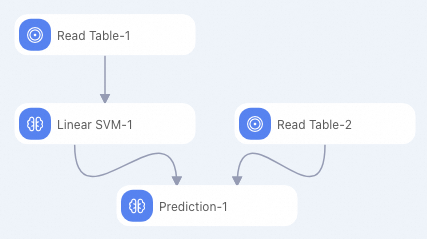
The Linear SVM component supports only a single input port that must be connected to the Read Table component.
Component parameters
Tab
Parameter
Required
Description
Fields Setting
Feature Columns
Yes
The input columns that are selected based on the characteristics of the input table. The data contained in the columns can be of the BIGINT or DOUBLE type.
Label Column
Yes
The label column that is selected based on the characteristics of the input table. The data contained in the column can be of the BIGINT, DOUBLE, or STRING type.
Parameters Setting
Positive Sample Label
No
The objective reference value. A random value is selected if you do not specify this parameter. If the difference between the positive example and negative example is large, we recommend that you specify this parameter.
Positive Penalty Factor
No
The weight of positive examples. Valid values: (0,+∞). Default value: 1.0.
Negative Penalty Factor
No
The weight of negative examples. Valid values: (0,+∞). Default value: 1.0.
Convergence Coefficient
No
The convergence deviation. Valid values: (0,1). Default value: 0.001.
Tuning
Cores
No
The number of cores that are used in computing. The system automatically allocates cores if this parameter is not specified.
Memory Size per Core
No
The memory size of each core. The system automatically allocates memory to each core if this parameter is not specified. Unit: MB.
Output ports
The Linear SVM component outputs binary models that have the same format as batch models to downstream prediction components by using output ports.
Method 2: Run Machine Learning Platform for AI commands
Configure the component parameters by using a Machine Learning Platform for AI command. You can use the SQL Script component to run Machine Learning Platform for AI commands. For more information, see SQL Script.
PAI -name LinearSVM -project algo_public
    -DinputTableName="bank_data"
    -DmodelName="xlab_m_LinearSVM_6143"
    -DfeatureColNames="pdays,emp_var_rate,cons_conf_idx"
    -DlabelColName="y"
    -DpositiveLabel="0"
    -DpositiveCost="1.0"
    -DnegativeCost="1.0"
    -Depsilon="0.001";
The following table describes the parameters that are used in the Machine Learning Platform for AI command.
Parameter | Required | Description | Default value |
inputTableName | Yes | The name of the input table. | None |
inputTablepartitions | No | The partition that is selected from the input table for training. The following formats are supported:
Note If you specify multiple partitions, separate them with commas (,). | All partitions |
modelName | Yes | The name of the output model. | None |
featureColNames | Yes | The feature columns that are selected from the input table for training. | None |
labelColName | Yes | The name of the label column in the input table. | None |
positiveLabel | No | The value of the positive example. | A random value that is selected from the values of label |
positiveCost | No | The weight of positive examples. It is also a positive penalty factor. Valid values: (0,+∞). | 1.0 |
negativeCost | No | The weight of negative examples. It is also a negative penalty factor. Valid values: (0,+∞). | 1.0 |
epsilon | No | The convergence coefficient. Valid values: (0,1). | 0.001 |
enableSparse | No | Specifies whether the input data is sparse. Valid values: true and false. | false |
itemDelimiter | No | The delimiter that is used to separate key-value pairs if data in an input table is sparse. | Comma (,) |
kvDelimiter | No | The delimiter that is used to separate keys and values if data in an input table is in sparse. | Colon (:) |
coreNum | No | The number of cores that are used in computing. The value of this parameter must be a positive integer. | Automatically allocated |
memSizePerCore | No | The memory size of each core. Valid values: 1 to 65536. Unit: MB. | Automatically allocated |
Example
Use the following training data as the input.
id
y
f0
f1
f2
f3
f4
f5
f6
f7
1
-1
-0.294118
0.487437
0.180328
-0.292929
-1
0.00149028
-0.53117
-0.0333333
2
+1
-0.882353
-0.145729
0.0819672
-0.414141
-1
-0.207153
-0.766866
-0.666667
3
-1
-0.0588235
0.839196
0.0491803
-1
-1
-0.305514
-0.492741
-0.633333
4
+1
-0.882353
-0.105528
0.0819672
-0.535354
-0.777778
-0.162444
-0.923997
-1
5
-1
-1
0.376884
-0.344262
-0.292929
-0.602837
0.28465
0.887276
-0.6
6
+1
-0.411765
0.165829
0.213115
-1
-1
-0.23696
-0.894962
-0.7
7
-1
-0.647059
-0.21608
-0.180328
-0.353535
-0.791962
-0.0760059
-0.854825
-0.833333
8
+1
0.176471
0.155779
-1
-1
-1
0.052161
-0.952178
-0.733333
9
-1
-0.764706
0.979899
0.147541
-0.0909091
0.283688
-0.0909091
-0.931682
0.0666667
10
-1
-0.0588235
0.256281
0.57377
-1
-1
-1
-0.868488
0.1
Use the following test data as the input.
id
y
f0
f1
f2
f3
f4
f5
f6
f7
1
+1
-0.882353
0.0854271
0.442623
-0.616162
-1
-0.19225
-0.725021
-0.9
2
+1
-0.294118
-0.0351759
-1
-1
-1
-0.293592
-0.904355
-0.766667
3
+1
-0.882353
0.246231
0.213115
-0.272727
-1
-0.171386
-0.981213
-0.7
4
-1
-0.176471
0.507538
0.278689
-0.414141
-0.702128
0.0491804
-0.475662
0.1
5
-1
-0.529412
0.839196
-1
-1
-1
-0.153502
-0.885568
-0.5
6
+1
-0.882353
0.246231
-0.0163934
-0.353535
-1
0.0670641
-0.627669
-1
7
-1
-0.882353
0.819095
0.278689
-0.151515
-0.307329
0.19225
0.00768574
-0.966667
8
+1
-0.882353
-0.0753769
0.0163934
-0.494949
-0.903073
-0.418778
-0.654996
-0.866667
9
+1
-1
0.527638
0.344262
-0.212121
-0.356974
0.23696
-0.836038
-0.8
10
+1
-0.882353
0.115578
0.0163934
-0.737374
-0.56974
-0.28465
-0.948762
-0.933333
Create the pipeline shown in the following figure. For more information, see Algorithm modeling.

Configure the parameters listed in the following table for the Linear SVM component. Retain the default values of the parameters that are not listed in the table.
Tab
Parameter
Description
Fields Setting
Feature Columns
Select the f0, f1, f2, f3, f4, f5, f6, and f7 columns.
Label Column
Select the y column.
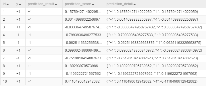
Run the pipeline and view the prediction results.
