Using the Swinging Door Trending Algorithm in PostgreSQL

This blog discusses Swinging Door Trending (SDT) algorithm and how you can use it in PostgreSQL for effective compression in Internet of Things applications.

By digoal

In Internet of Things (IoT) scenarios where monitoring and sensors are involved, data is constantly generated over time in streaming applications with large or even extreme amounts of data is recorded. For example, in performance monitoring scenarios, a curve that indicates performance is drawn based on several data points that are collected and recorded over time. These sorts of applications are now common in several industries nowadays, especially the IT, medicine, and finance sectors.

Now, imagine that if each sensor or metric involved in these IoT applications generates 1 point every 100 milliseconds, which in turn means that 864,000 points are generated on a daily basis. Now consider that there are several, or even several thousand or even millions of, sensors or metrics involved in such an application. For example, there may be a scenario in which one million sensors or metrics generate nearly 100 million data points a day. If you want to draw a graph for a period of time, it will take a long time to render such a multitude of data points.

With all that said, a good compression algorithm is extremely important when it comes to any IoT scenarios that involve continuous monitoring and large amounts of data points. So the question arises are there compression algorithms available that can help with all of this but also ensure that the data is not distorted in the process? If so, which algorithms are they?

To answer this question, in this blog, we will show you the Swinging Door Trending (SDT) algorithm and how you can use it in PostgreSQL for effective compression in IoT scenarios.

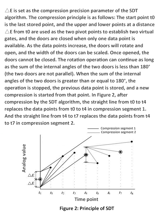
The Swinging Door Trending Algorithm

The Swinging Door Trending (SDT) algorithm is a linear trend compression algorithm. In essence, it replaces a series of continuous data points with a straight line determined by the start and end points.

The algorithm needs to record the length of each time interval, the data of the start point and the data of the end point. The data of the end point for the previous segment is the data of the start point for the next segment.

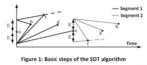
The basic principle is relatively simple, please see the figure.

The first data point "a" has one point above and one point below. The distance between them and "a" is E (that is, the width of the door). These two points serve as the two pivot points of the "door". When only the first data point is available, both doors are closed. As the number of points increases, the doors will open gradually. Note that the width of each door can be scaled, and within a certain period of time, once a door is opened, it cannot be closed.

As long as the two doors are not parallel, or the sum of the two inner angles is less than 180° (the algorithm in this article uses this point to judge), this "swinging door" operation can continue. In the figure, the first time interval is from "a" to "e". The result is that the straight line from "a" to "e" are used to replace the data points (a, b, c, d, e), and it plays a role in controlling the compression distortion (E).

The second interval starts from the point "e". At the beginning, the two doors are closed and gradually opened. The subsequent operation is similar to that of the previous interval.

Use the SDT Algorithm in PostgreSQL

Based on the principle of the SDT algorithm, several required input items can be known.

Points with x and y coordinates (if they are points on the timeline, they can be converted into this form by epoch).
E, the width of the door, plays a role in controlling the compression distortion.

You can use the algorithm in PostgreSQL to do the following:

1. Create a test table.

create table tbl(id int, -- ID, optional
val numeric, -- value (such as the point value of a sensor or the financial industry)
t timestamp  -- value timestamp
);

2. Insert 100,000 pieces of test data.

insert into tbl select generate_series(1,100000), round((random()*100)::numeric, 2), clock_timestamp()+(generate_series(1,100000) || ' second')::interval ; 

test=> select * from tbl limit 10;
 id |  val  |             t              
----+-------+----------------------------
  1 | 31.79 | 2016-08-12 23:22:27.530318
  2 | 18.23 | 2016-08-12 23:22:28.530443
  3 |  5.14 | 2016-08-12 23:22:29.530453
  4 | 90.25 | 2016-08-12 23:22:30.530459
  5 |  8.17 | 2016-08-12 23:22:31.530465
  6 | 97.43 | 2016-08-12 23:22:32.53047
  7 | 17.41 | 2016-08-12 23:22:33.530476
  8 |  0.23 | 2016-08-12 23:22:34.530481
  9 | 84.67 | 2016-08-12 23:22:35.530487
 10 | 16.37 | 2016-08-12 23:22:36.530493
(10 rows)

3. Convert time to the value on the x axis, supposing that every 1 second is 1 unit of the x coordinate.

test=> select (extract(epoch from t)-extract(epoch from first_value(t) over())) / 1 as x,  -- divided by 1 second as 1 unit
val, t from tbl limit 100;
        x         |  val  |             t              
------------------+-------+----------------------------
                0 | 31.79 | 2016-08-12 23:22:27.530318
 1.00012493133545 | 18.23 | 2016-08-12 23:22:28.530443
 2.00013494491577 |  5.14 | 2016-08-12 23:22:29.530453
 3.00014090538025 | 90.25 | 2016-08-12 23:22:30.530459
 4.00014686584473 |  8.17 | 2016-08-12 23:22:31.530465
 5.00015187263489 | 97.43 | 2016-08-12 23:22:32.53047
 6.00015807151794 | 17.41 | 2016-08-12 23:22:33.530476
 7.00016307830811 |  0.23 | 2016-08-12 23:22:34.530481
 8.00016903877258 | 84.67 | 2016-08-12 23:22:35.530487

4. Compile a function to implement the SDT algorithm.

create or replace function f (
  i_radius numeric,       --  compression radius
  i_time timestamp,       --  start time
  i_interval_s numeric,   --  time conversion interval in seconds (for example, every 5 seconds indicates 1 unit interval on the coordinate, then 5 is used here) 
  query text,             --  data that requires to be compressed by the SDT algorithm. For example, "select t, val from tbl where t>=%L order by t limit 100", where the select clause must be fixed, and be sorted by  t
  OUT o_val numeric,      --  value, vertical coordinate y (skip point y)
  OUT o_time timestamp,   --   time, horizontal coordinate x (skip point x)
  OUT o_x numeric         --  skip point x, converted by o_time
)
returns setof record as 
$$

declare
  v_time timestamp;       -- time variable
  v_x numeric;            -- convert v_time to v_x
  v_val numeric;          -- y coordinate
  v1_time timestamp;      -- time variable of the previous point
  v1_x numeric;           -- convert v_time to v_x for the previous point
  v1_val numeric;         -- y coordinate of the previous point
  v_start_time numeric;   -- record the time coordinate of the start point, used to compute the x offset
  v_rownum int8 := 0;     -- used to mark whether it is the first row
  v_max_angle1 numeric;   -- maximum angle of the upper door
  v_max_angle2 numeric;   -- maximum angle of the lower door
  v_angle1 numeric;       -- included angle of the upper door
  V_angle2 numeric; -- included angle of the lower door
begin
  for v_time , v_val in execute format(query, i_time) 
  LOOP
    -- The first point in the first line is the actual point to be recorded
    v_rownum := v_rownum + 1;
    if v_rownum=1 then 
      v_start_time := extract(epoch from v_time);  
      v_x := 0;  
      o_val := v_val;  
      o_time := v_time;  
      o_x := v_x;  
      -- raise notice 'rownum=1 %, %', o_val,o_time;
      return next;  -- return the first point  
    else
      v_x := (extract(epoch from v_time) - v_start_time) / i_interval_s;  -- generate the x coordinate
      SELECT 180-ST_Azimuth(
                              ST_MakePoint(o_x, o_val+i_radius),    -- the point on the upper door
                              ST_MakePoint(v_x, v_val)              -- next point
                           )/(2*pi())*360 as degAz,                 -- the upper included angle
                 ST_Azimuth(
                              ST_MakePoint(o_x, o_val-i_radius),    -- the point on the lower door
                              ST_MakePoint(v_x, v_val)              -- next point
                           )/(2*pi())*360 As degAzrev               -- the lower included angle
      INTO v_angle1, v_angle2; 

      select GREATEST(v_angle1, v_max_angle1), GREATEST(v_angle2, v_max_angle2) into v_max_angle1, v_max_angle2;

      if (v_max_angle1 + v_max_angle2) >= 180 then  -- find the point outside the quadrilateral, output the previous point, and recompute the quadrilateral from the previous point
        -- raise notice 'max1 %, max2 %', v_max_angle1 , v_max_angle2;
        -- recover
        v_angle1 := 0;
        v_max_angle1 := 0;
        v_angle2 := 0;
        v_max_angle2 := 0;

        -- The door has been fully opened, and the value of the previous point is output
        o_val := v1_val; 
        o_time := v1_time; 
        v1_x := (extract(epoch from v1_time) - v_start_time) / i_interval_s;  -- generate the x coordinate of the previous point 
        o_x := v1_x; 

        -- Use a new door, and compute the new included angle between the door and the current point. 
        SELECT 180-ST_Azimuth(
                                ST_MakePoint(o_x, o_val+i_radius),    -- the point on the upper door
                                ST_MakePoint(v_x, v_val)              -- next point
                             )/(2*pi())*360 as degAz,                 -- the upper included angle
                   ST_Azimuth(
                                ST_MakePoint(o_x, o_val-i_radius),    -- the point on the lower door
                                ST_MakePoint(v_x, v_val)              -- next point
                             )/(2*pi())*360 As degAzrev               -- the lower included angle
        INTO v_angle1, v_angle2;

        select GREATEST(v_angle1, v_max_angle1), GREATEST(v_angle2, v_max_angle2) into v_max_angle1, v_max_angle2; 

        -- raise notice 'new max %, new max %', v_max_angle1 , v_max_angle2;

        -- raise notice 'rownum<>1 %, %', o_val, o_time;

        return next;
      end if; 

      -- Record the current value, and save it as the previous point of the next point
      v1_val := v_val; 
      v1_time := v_time; 
    end if; 
  END LOOP; 
end; 

$$
 language plpgsql strict;

5. Complete a compression test. To do this, set the door width is 15 and the start point is "2016-08-12 23:22:27.530318". Every second represents one unit on the x coordinate.

test=> 
select * from f (
  15, -- door width = 15
  '2016-08-12 23:22:27.530318', -- start time
  1, -- interval of the conversion from time to coordinate, which is 1 second
  'select t, val from tbl where t>=%L order by t limit 100'  -- query
);

 o_val |           o_time           |       o_x        
-------+----------------------------+------------------
 18.23 | 2016-08-12 23:22:28.530443 |                0
  5.14 | 2016-08-12 23:22:29.530453 | 1.00001287460327
 90.25 | 2016-08-12 23:22:30.530459 | 2.00001883506775
......
 87.90 | 2016-08-12 23:24:01.53098  | 93.0005400180817
 29.94 | 2016-08-12 23:24:02.530985 | 94.0005450248718
 63.53 | 2016-08-12 23:24:03.53099  | 95.0005497932434
 12.25 | 2016-08-12 23:24:04.530996 | 96.0005559921265
 83.21 | 2016-08-12 23:24:05.531001 | 97.0005609989166
(71 rows)

From the above example, we can see that 100 points are compressed into 71 points. The following are the values of the original 100 points:

test=> select val, t, (extract(epoch from t)-extract(epoch from first_value(t) over()))/1 as x from tbl where t>'2016-08-12 23:22:27.530318' order by t limit 100;
  val  |             t              |        x         
-------+----------------------------+------------------
 18.23 | 2016-08-12 23:22:28.530443 |                0
  5.14 | 2016-08-12 23:22:29.530453 | 1.00001001358032
 90.25 | 2016-08-12 23:22:30.530459 |  2.0000159740448
......
 83.21 | 2016-08-12 23:24:05.531001 | 97.0005581378937
 87.97 | 2016-08-12 23:24:06.531006 | 98.0005631446838
 58.97 | 2016-08-12 23:24:07.531012 | 99.0005691051483
(100 rows)

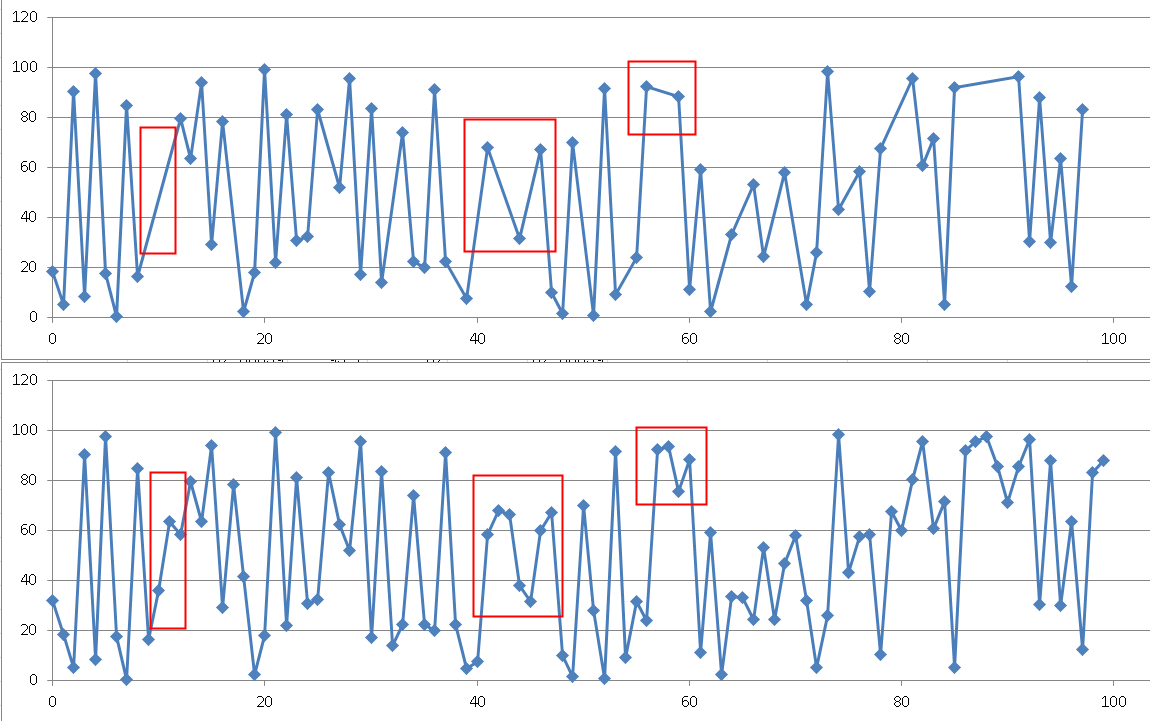
Next, use Excel to draw a graph for the comparison before and after compression.

In the above figure, the upper one of the two is the data graph after compression, and the lower one is the data graph before compression. The position marked in red is the data compressed by the SDT algorithm. In this application, distortion is completely under control.

Use the Algorithm for Effective Compression

You can additionally modify the function to create a function with an array as the input parameter. In the form of lambda, the data can be retrieved from the continuous stream input pipeline in real time, and run from there. To do this, you can use one of either two methods.

1. Create an Async Batch Consume with Atomicity operation.

In the stream computing result table (valid point), add 2 fields: Add the PK, which is to be associated with the detail table and the timestamp, which indicates the last record. The Async Batch Consume with Atomicity operation will start from the last valid point to continue consuming data from the detail table.

2. Update the status directly on the detail table. That is, update the status to as whether the point and current record are visible.

All others involving intermediate computations can be implemented in a similar way. That is, when computing the current record, you can update the computation results to the current record. You can do this through the stream computing method of directly updating the detail table. If you need to use the previous stream computing results during computation, it is easy to obtain them through recursion or using UDF calls.

For example:

Create detail table (
  Definition of reported content fields ....,
  Intermediate result field ....,
  Visibility field ....
);

It can also be written as an aggregate function that is called in the PostgreSQL-based stream database pipelineDB to implement stream computing.

Summary

By using the SDT algorithm, you can compress continuously generated data in streaming applications in real time. This can be useful to IoT scenarios in a variety of industries, such as IT, ecology, security, or medicine, which require real-time data monitoring and data streaming.

The SDT algorithm allows data to be computed and compressed in the database without being loaded from the database. Users can also compress streaming data based on their needs. Similarly, the data does not need to be loaded from the database, and can be completed on the database side.

So, in conclusion, PostgreSQL along with SDT algorithm provides a powerful solution to maintain the massive amounts of data in monitoring scenarios.

Community

Using the Swinging Door Trending Algorithm in PostgreSQL

The Swinging Door Trending Algorithm

Use the SDT Algorithm in PostgreSQL

Use the Algorithm for Effective Compression

Summary

References

Read previous post:

Read next post:

digoal

You may also like

Comments

digoal

Related Products

IoT Platform

IoT Solution

AnalyticDB for PostgreSQL

Global Internet Access Solution