DeepRec: A Training and Inference Engine for Sparse Models in Large-Scale Scenarios

This article will introduce DeepRec in the following three aspects:

Background (Why we propose DeepRec)
Features (Design purpose and implementation)
DeepRec Community (Major features of the latest released 2206 version)

Background

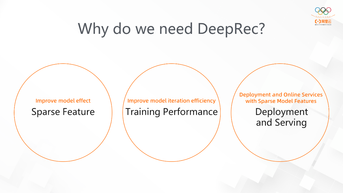
Why do we need DeepRec? The current community version of TensorFlow supports sparse scenarios, but it has some shortcomings in the following three aspects:

The training function that can improve the sparse model effect
The training performance that can improve the sparse model iteration efficiency
The deployment of sparse models

Therefore, we proposed DeepRec, which was designed to perform depth optimization in sparse scenarios.

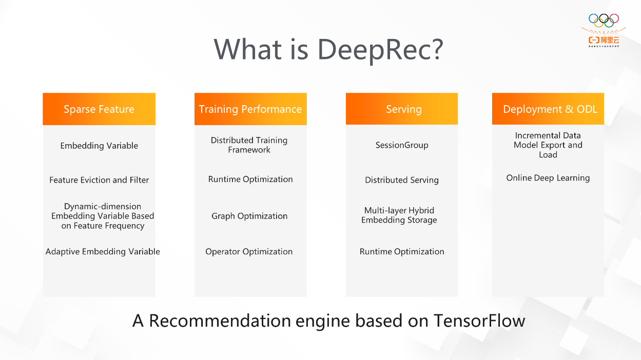
DeepRec has four main features: embedding, training performance, serving, and deployment & ODL.

DeepRec mainly supports the following core businesses in Alibaba (including recommendation, search, and advertising). We also provide some cloud customers with solutions in some sparse scenarios. It significantly improves their model effect and iteration efficiency.

Features

The features of DeepRec contain the following five main aspects: embedding, training framework (asynchronous training framework and synchronous training framework), Runtime (Executor and PRMalloc), graph optimization (structured model and SmartStage), and Serving-related features.

1. Embedding

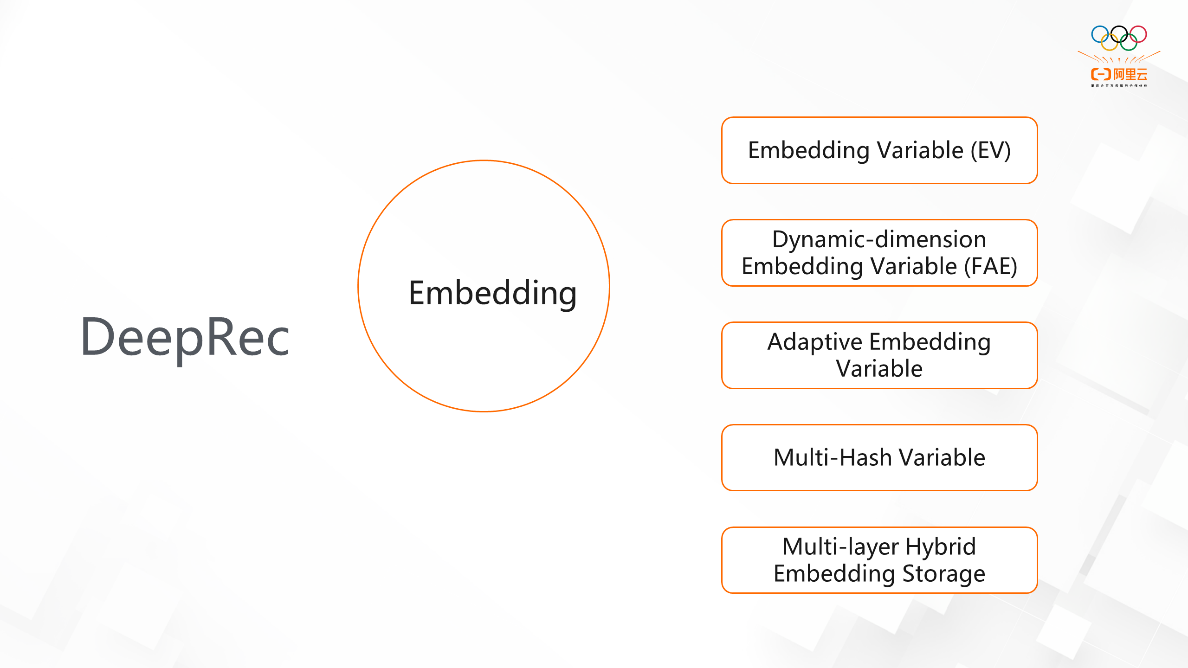
For the Embedding feature, five sub-features will be introduced:

1.1 Embedding Variable (EV)

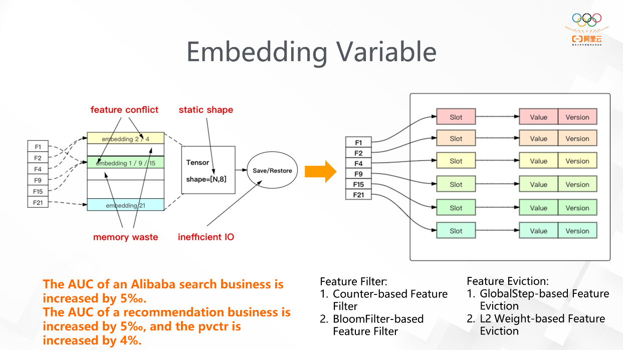
The left part of the figure above shows the main way in which TensorFlow supports the Embedding feature. Users define the Tensor with the static shape, and the sparse features are mapped to the just-defined Tensor by Hash + Mod. However, there are four problems:

Feature Conflict: Hash + Mod tends to introduce feature conflicts, which will lead to the disappearance of effective features and thus impair the effect.
Memory Waste: For storage, this method will lead to memory waste, as some memory space will not be used.
Static Shape: Once the shape of the Variable is static, it cannot be changed.
Inefficient I/O: If users define the Variable this way, it must be exported in full. If the dimension of the Variable is large, it is very time-consuming to export or load it but changes are limited in sparse scenarios.

In this case, the design principle of EmbeddingVariable defined by DeepRec is to convert static Variable into dynamic HashTable-like storage and create a new Embedding for each key, thus solving feature conflicts. However, due to this design principle, when there are many features, a large amount of memory will be consumed because of the disordered expansion of EmbeddingVariable. Therefore, DeepRec introduces the following two features: feature filter and feature eviction. These two features can effectively filter low-frequency features and evict features that are not helpful for training. In sparse scenarios (such as search and recommendation), some long-tail features have little model training. Therefore, feature filters (such as CounterFilter and BloomFilter) set a threshold for features to enter EmbeddingVariable. The feature eviction triggers feature elimination every time checkpoint is saved, and features with older timestamps will be eliminated. The AUC of a recommendation business is increased by 5‰ in Alibaba, the AUC of a recommendation business is increased by 5‰ in Alibaba Cloud, and the pvctr is increased by 4%.

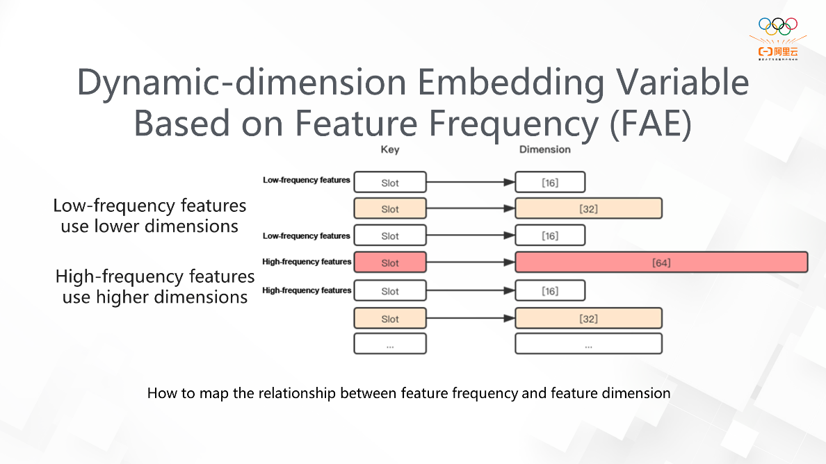
1.2 Dynamic-Dimension Embedding Variable Based on Feature Frequency (FAE)

Typically, the EmbeddingVariable corresponding to the same feature is set to the same dimension. If the EmbeddingVariable is set to a higher dimension, the low-frequency feature is prone to cause overfitting and consumes a lot of memory. Conversely, if the EmbeddingVariable is set to a lower dimension, high-frequency features may affect the model effect due to insufficient expression. The FAE function provides different dimensions for the same feature according to different feature frequencies. The model is trained automatically, so the model effect can be guaranteed, and the resources for training can be saved. This is an introduction to the FAE function. The function allows users to introduce a dimension and statistical algorithm, and then FAE automatically generates different EmbeddingVariable according to the implemented algorithm. DeepRec will adaptively discover and assign dimensions to features within the system in the future, thus improving user usability.

1.3 Adaptive Embedding Variable

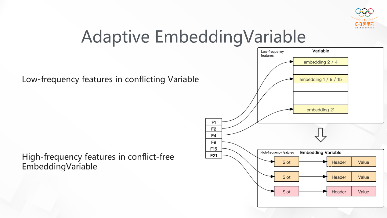
This feature is similar to the second feature in that both focus on defining the relationship between Variables and high-frequency or low-frequency features. When the EV dimension mentioned above is particularly large, much memory is occupied. In Adaptive Embedding Variable, we use two Variables, as shown in the right half of the figure. We define one of the Variables as static, and the low-frequency features will be mapped to this Variable as much as possible. The other is defined as the dynamic-dimension Embedding Variable mapped with high-frequency features. Variable supports the dynamic conversion of low-frequency and high-frequency features, which significantly reduces the memory occupied by the system. For example, after training, the first dimension of a certain feature may be close to 1 billion, while only 20%-30% of the features are important. In this adaptive way, such a large dimension is not required, thus significantly reducing the use of memory. In practice, we found that the effect on the accuracy of the model is very small.

1.4 Multi-Hash Variable

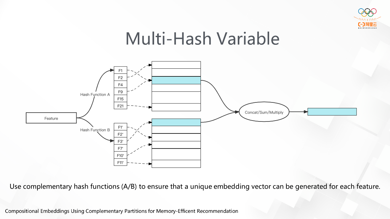
This feature is to solve feature conflicts. We used to solve feature conflicts by using Hash + Mod. Now, we use two or more Hash and Mod functions to get Embedding and then perform Reduction on the obtained Embedding. The advantage is that we can solve feature conflicts with less memory use.

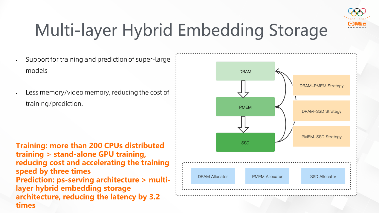
1.5 Multi-Layer Hybrid Embedding Storage

This function is also designed for situations where EV has a large number of features, and much memory is occupied. The memory occupied by workers may be tens or hundreds of GB during training. We find that the features follow a typical power-law distribution. Considering this characteristic, we put high-frequency features into more precious resources (such as CPU), while relatively long-tail and low-frequency features are put into cheaper resources. As shown in the right half of the figure, there are three structures: DRAM, PMEM, and SSD. PMEM is provided by Intel, with speed between DRAM and SSD, but it has a large capacity. We support a hybrid storage of DRAM-PMEM, DRAM-SSD, and PMEM-SSD, and we also achieve some business fruits. There is a business on the cloud that previously used more than 200 CPUs for distributed training, but now, the training mode is changed to stand-alone GPU training after multi-layer storage is adopted.

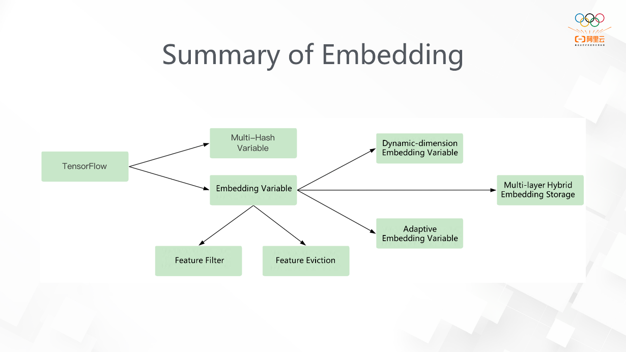
That's all for the introduction to all the sub-features of Embedding. These features are designed to solve several problems in TensorFlow (mainly feature conflicts). Our solutions are Embedding Variable and Multi-Hash Variable. We have developed feature filter and feature eviction features to reduce the large memory overhead of Embedding Variable. In terms of feature frequency, we have developed three features: Dynamic-dimension Embedding Variable, Adaptive Embedding Variable, and Multi-Layer Hybrid Embedding Storage. The first two solve problems from the perspective of dimension, and the last one solves problems from the perspective of software and hardware.

2. Training Framework

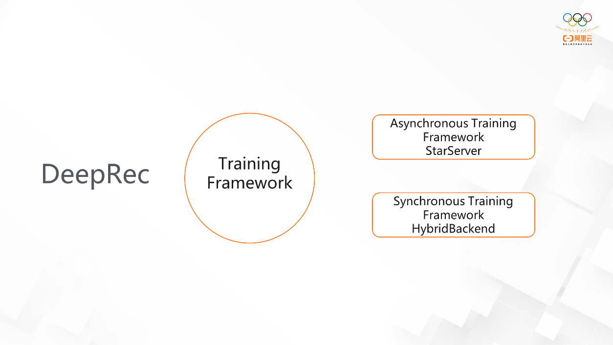
The second part is the training framework. It can be introduced in two aspects: asynchronous training framework and synchronous training framework.

2.1 Asynchronous Training Framework: StarServer

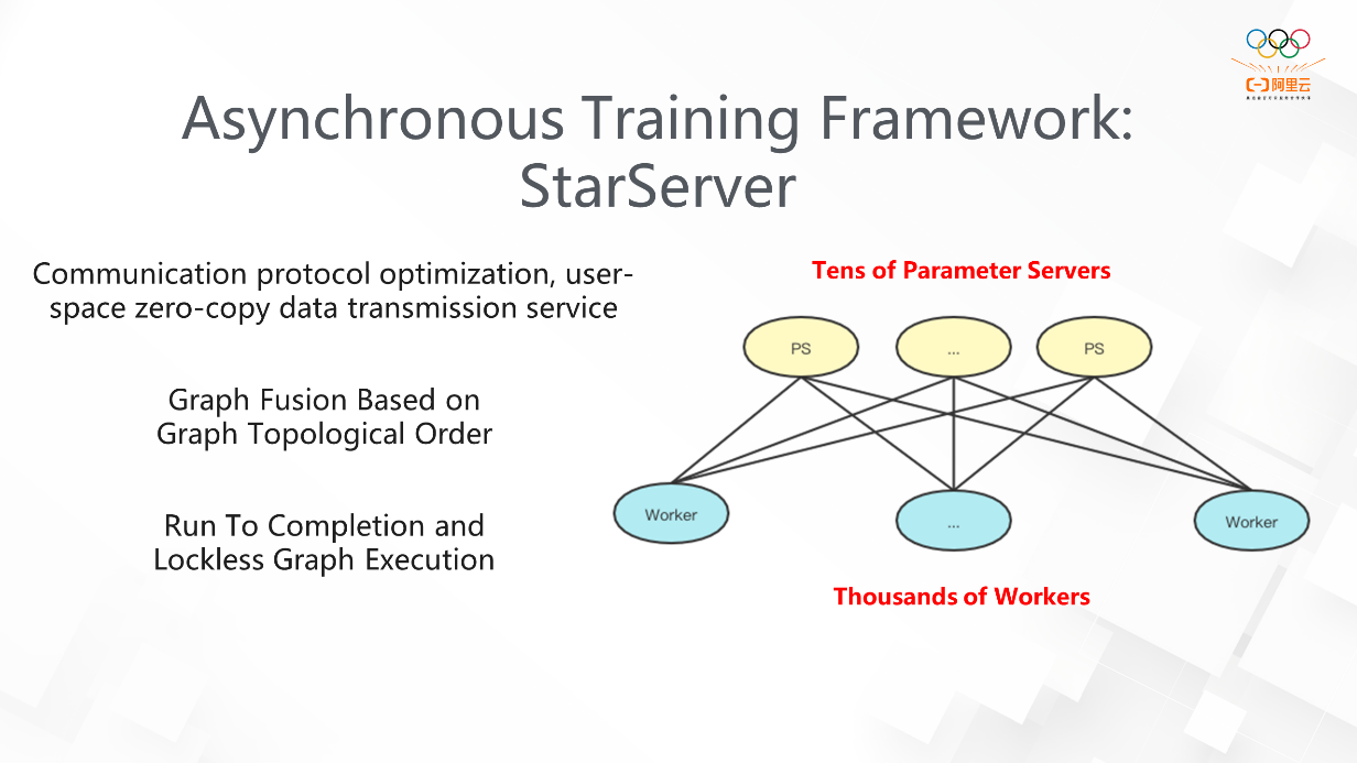
Some problems in TensorFlow are exposed in large-scale jobs (hundreds or thousands of workers), such as inefficient thread pool scheduling, high overhead on multiple critical paths, and frequent small-packet communications. All these problems have become the bottleneck of distributed communication.

StarServer has done a good job in graphs, thread pool scheduling, and memory optimization. The send/recv semantics in TensorFlow is changed to pull/push semantics. In StarServer, we optimize the runtime of ParameterServer (PS) with share-nothing architecture and lockless graph execution. Compared with the performance of the native framework, the performance of StarServer has been improved several times, and we can achieve linear expansion when the number of internal workers is about 3,000.

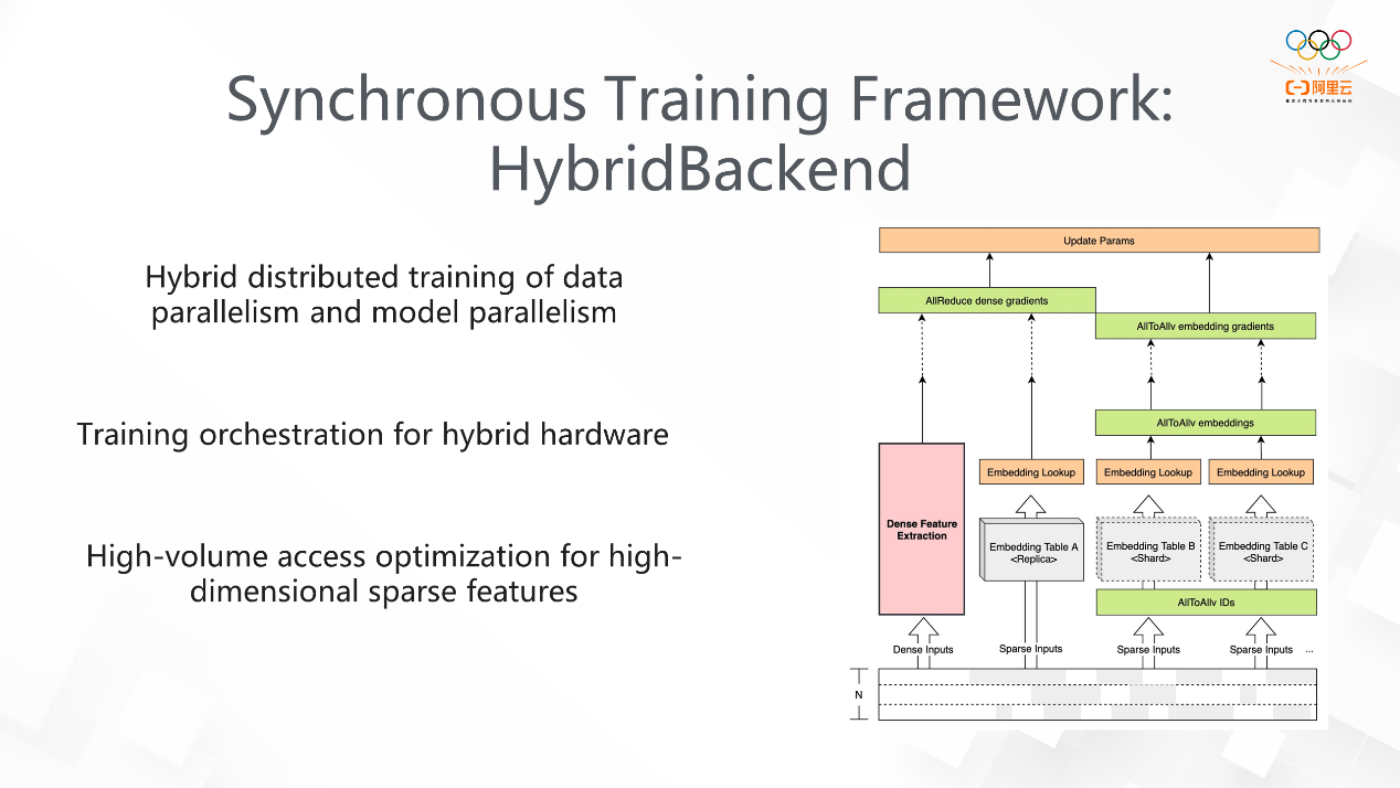
2.2 Synchronous Training Framework: HybridBackend

This is the solution we developed for synchronous training. It supports hybrid distributed training of data parallelism and model parallelism. Data reading is completed through data parallelism. Model parallelism supports training with a large number of parameters and uses data parallelism for dense matrix computing. According to the characteristics of EmbeddingLookup, we have done the merging and grouping optimization of multi-way Lookup and used the advantages of GPU Direct RDMA to design the whole synchronous framework based on the network topology awareness.

3. Runtime

The third major feature is Runtime. I will focus on introducing PRMalloc and Executor optimization.

3.1 PRMalloc

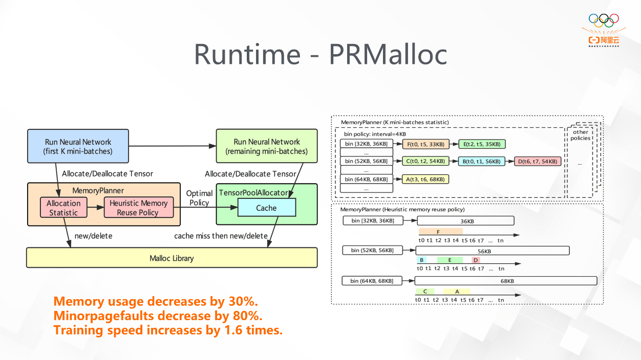
The first is memory allocation optimization. Memory allocation is ubiquitous in both TensorFlow and DeepRec. The first thing we found in sparse training is that large memory allocation causes a large number of minorpagefaults. In addition, there are concurrent allocation problems in multi-threaded allocation. In DeepRec, based on the forward and backward calculations of sparse training, we designed a memory allocator for deep learning called PRMalloc. It improves memory usage and system performance. As you can see in the figure, the main part is MemoryPlanner. It is used to count the characteristics of the current training in the mini-batches statistic of the first k rounds of model training and collect the tensor allocation information during execution. MemoryPlanner needs to record the information with bin buffer and optimize them accordingly. After k rounds, we apply it, significantly reducing the problems above. We found that this can significantly reduce minorpagefaults, reduce memory usage, and speed up training by 1.6 times when using DeepRec.

3.2 Executor Optimization

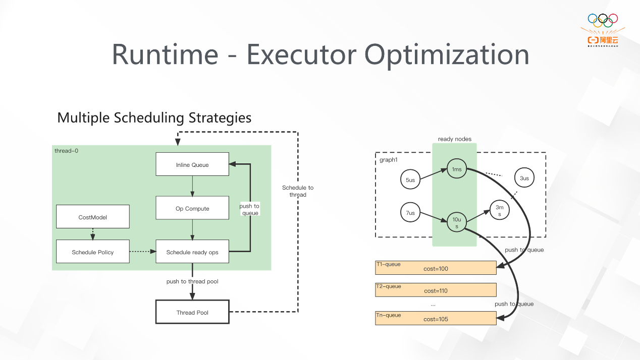
The implementation of TensorFlow's native Executor is simple. First, perform a topological sort on DAG, insert Node into the execution queue, and use Executor to do scheduling with Task. However, this implementation does not take the actual business characteristics into account. The Eigen thread pool is used by default. If the load on the thread is uneven, work stealing will occur in a large number of threads, resulting in great overhead. In DeepRec, we define more even scheduling and define the critical path at the same time, so there is a certain priority during scheduling to execute Op. Finally, DeepRec provides a variety of scheduling policies based on Task and SimpleGraph.

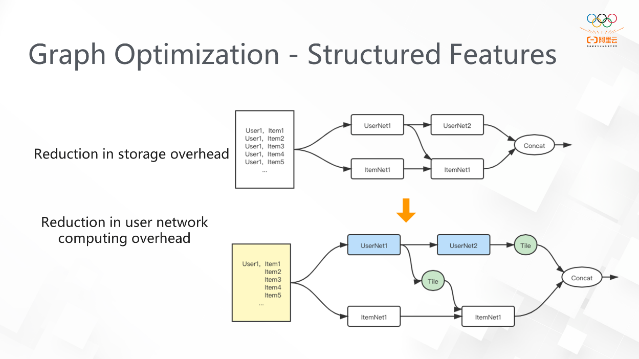
4. Functions Related to Graph Optimization

4.1 Structured Features

This is a feature inspired by business. We found that in search scenarios, whether it is training or inference, the sample is often one user corresponding to multiple items and multiple labels. This kind of sample is saved as multiple samples in the original processing method, so the storage of the user is redundant. In order to save this memory overhead, we customize the storage format to optimize this part. If these samples contain the same user in a minibatch, some user networks and item networks will perform calculations separately. Finally, the corresponding logical computing will be finished. This method can save computing costs. Therefore, we have made structural optimization in storage and computing, respectively.

4.2 SmartStage

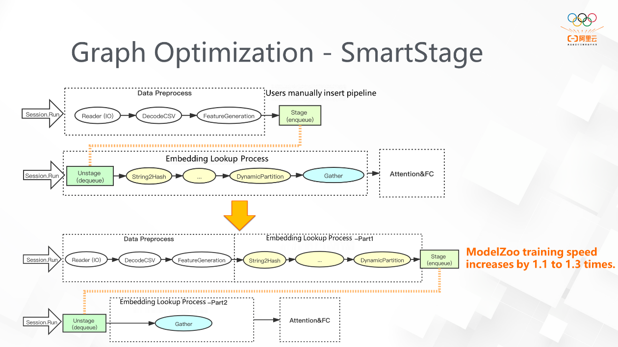
As we can see, the training of sparse models usually includes sample reading, EmbeddingLookup, and MLP network computing. Sample reading and EmbeddingLookup are not compute-intensive, so computing resources cannot be used efficiently. Although the prefetch interface provided by the native framework can complete asynchronous operations to some extent, the complex subgraphs we designed in the EmbeddingLookup process cannot be pipelined using the prefetch of TensorFlow. The pipeline feature provided by TensorFlow requires the user to display the specified stage boundary in actual use. On the one hand, it will make it more difficult to use. On the other hand, due to the insufficient precision of the stage, it cannot be as accurate as the Op level. Manual insertion is impossible for high-level API users, which will lead to the parallelization of many steps. The following figure shows the specific operations of SmartStage. It automatically classifies Ops into different stages to improve the performance of concurrent pipelines. In ModelZoo, the test result shows that the maximum speedup ratio of our model can reach 1.1-1.3.

5. Serving

5.1 Incremental Data Model Export and Load

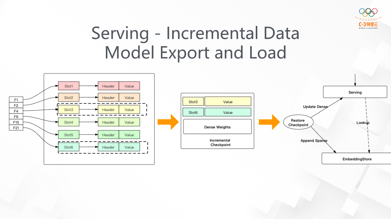
In the beginning, when we introduce Embedding, one of the important points is inefficient I/O. If the aforementioned Embedding Variable is applied, we can do incremental export. As long as the sparse ID that has been accessed is added to the graph, the ID that we need can be accurately exported during incremental export. We have two purposes to design this feature. First, our original method for model training exports the full model in each step, and it restores checkpoint when the program interrupts. At worst, we may lose all the results in the two checkpoint intervals. With incremental export, we will export the dense part in full, and incremental export is adopted for the sparse part. In the actual scenario, the incremental export in ten minutes can save the loss caused by restoring. In addition, the incremental export scenario is online serving. If a model is loaded in full every step, the model is large in sparse scenarios, and each load takes a long time. It will be difficult for online learning, so incremental export will also be used in the ODL scenario.

5.2 ODL

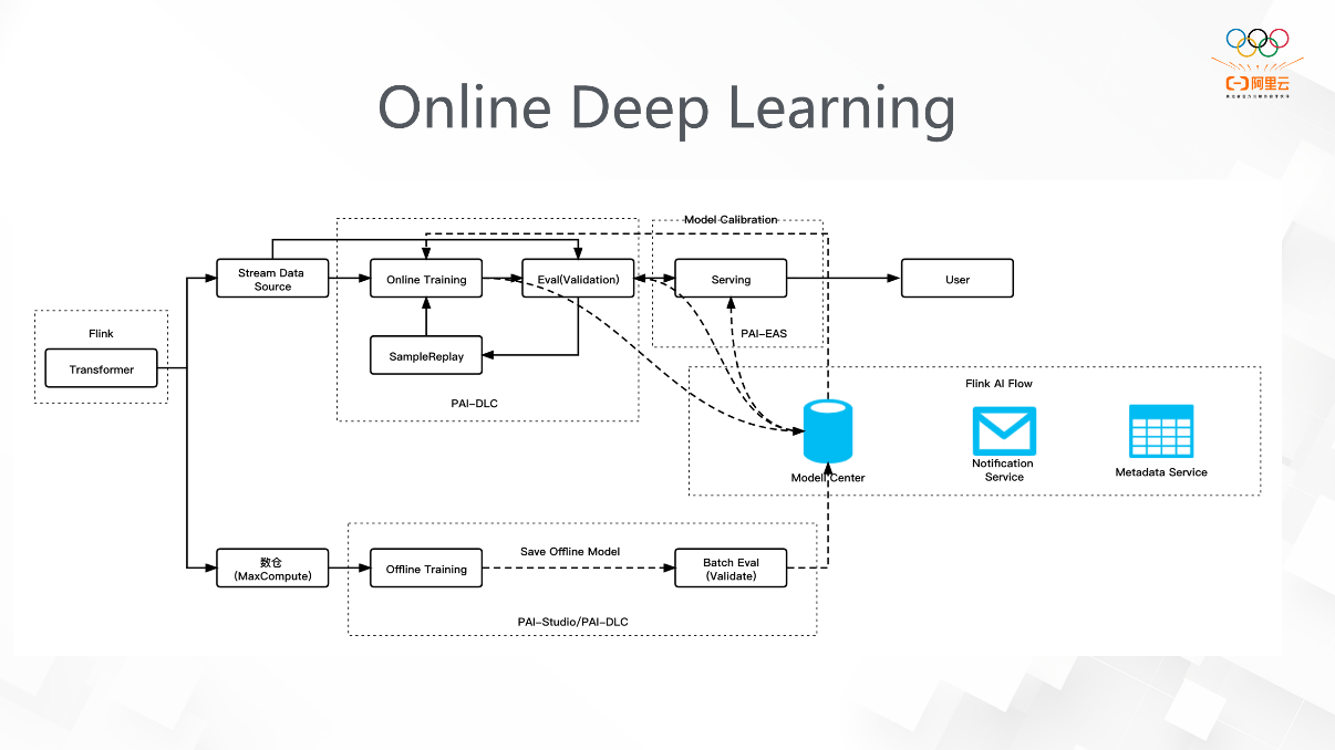
The leftmost part is sample processing, the upper and lower parts are offline and online training, and the right part is serving. Many PAI components are used to construct the pipeline.

DeepRec Community

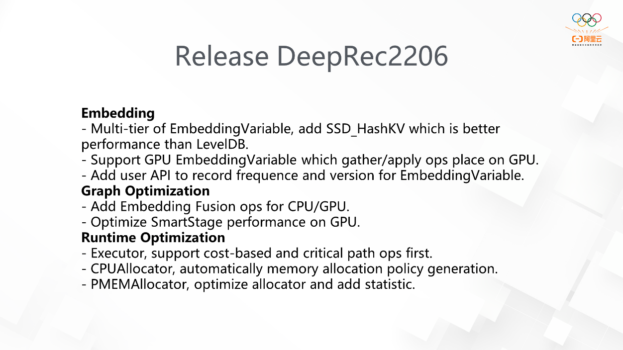
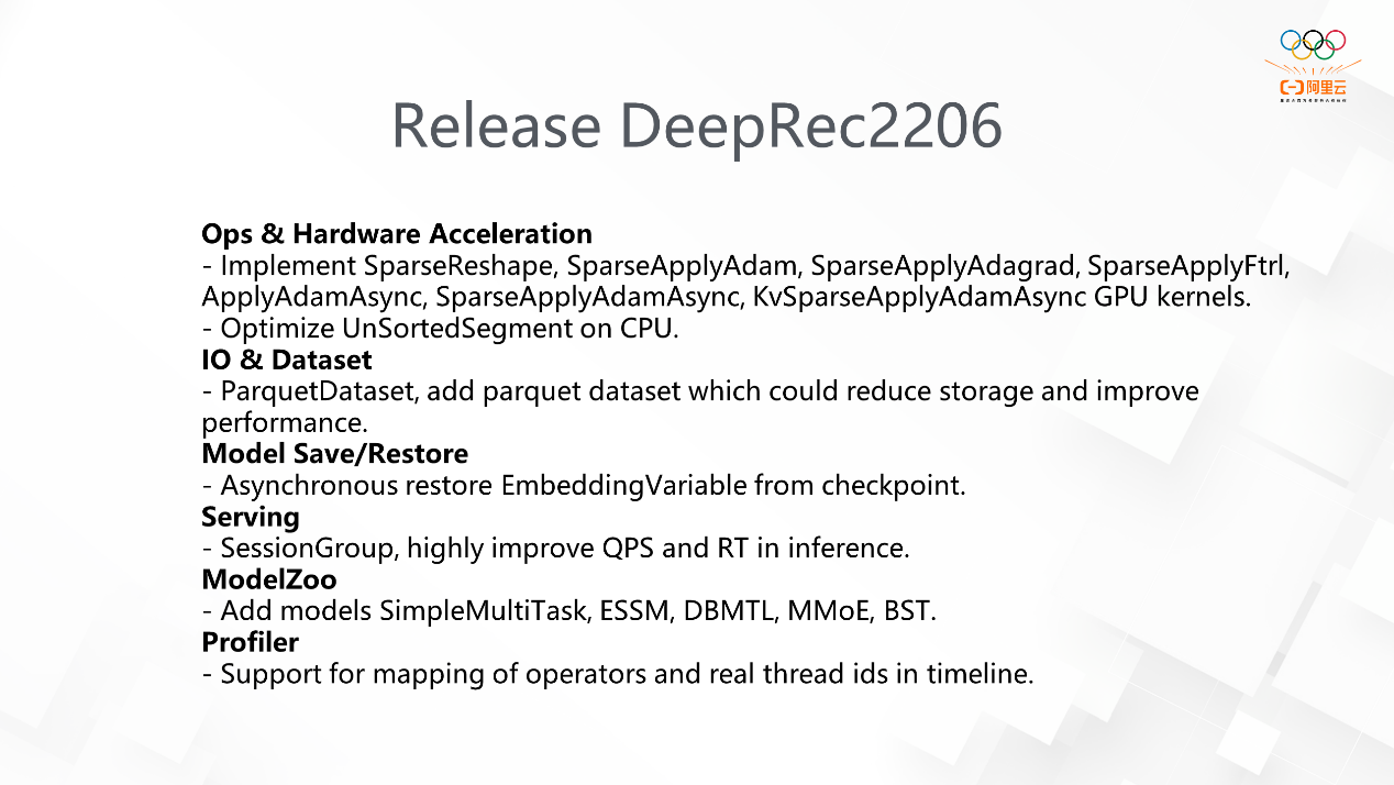
In terms of community, we released a new version 2206 in June 2022. It mainly includes the following new features:

Community